

1 Introduction
Bio-arrays yield a new type of medical imaging. In this note, an algorithm based on differential geometry for automatic analysis of bio-arrays is proposed. The method may be eventually efficient to treat other types of images. The algorithm uses elementary metric properties of surfaces and differential systems techniques. It was tested on bio-arrays imaging (provided by the INSERM team of F. Berger and E. Chambaz) versus other image processing techniques as ‘watershed lines’.
This note comprises three parts: a presentation of the experimental protocol that explains some of the special features of bio-arrays imaging, followed by the presentation of the algorithm and of its results, and it ends with conclusion and perspectives.
2 A differential geometry approach to automatic analysis of bio-arrays
2.1 Bio-arrays, experimental protocol and type of image
Since a few years, different techniques are used to detect diseases; they are known under the name of micro-arrays, macro-arrays, DNA chips; they differ mainly on the scale of applications. All these techniques are jointly referred to under the common name of bio-arrays. Implementation of these chips relies on genome cartography and aims at quantifying genes under study at some stage of the development of the cell. There are two techniques most frequently used with bio-arrays. The Multiplex Messenger Assay relies on a radioactivity analysis and the National Human Genome Research Institute uses fluorescence. In the second case, images have several colours channels, but this makes no difference for the algorithm.
First step for each gene under study selects the complementary sequence cDNA. These cDNAs are replicated in high quantity and then fixed on a film. On this film, all cDNAs of the same type are localised at the same place. The second step takes mRNA out of the substrate. These mRNAs are produced by reverse transcription isotopic single strand 33PDNAs in such a way that A, C, T, G are replaced with radioactive equivalent bases. The last step displays these radioactive sequences on the film where they fix the corresponding sequences of cDNA (cf. Fig. 1). The image is produced out of radioactivity or fluorescence and displays several spots (also named ‘mesas’ or peaks).
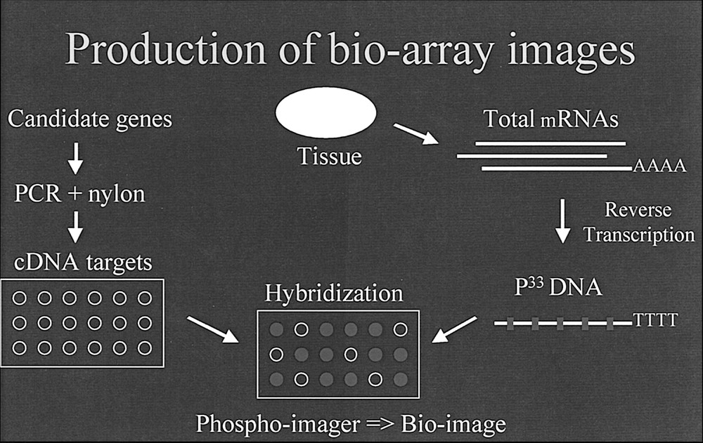
The principles of production of bio-array images.
2.2 A new segmentation method
The first application of a differential geometry approach in medical imaging has been reported in 〚1, 2〛; it has also been already proposed to use a potential-Hamiltonian system for medical image enhancement 〚3–5〛. The present approach combines both types of concepts of differential geometry and dynamical systems theory in order to obtain a new tool for the segmentation of medical images. Let g(x,y) be the height function that associates to a pixel of coordinates (x,y) the level of the image at this point. The first processing consists in filtering the initial image by using a low-pass filter (Fig. 2).
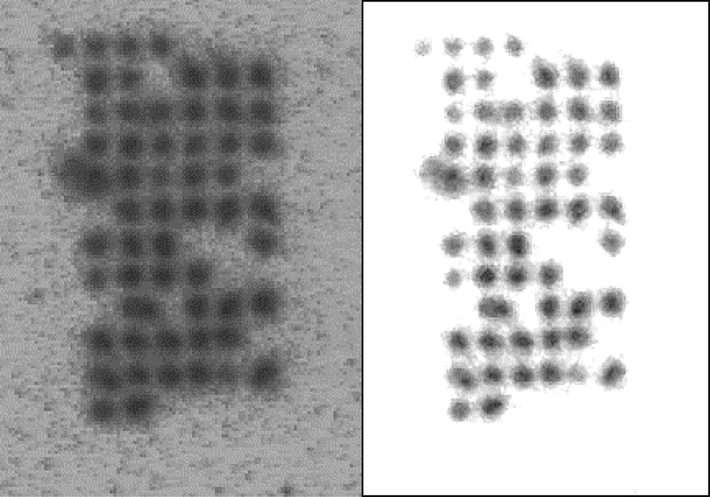
Initial bio-array image (left) and image treated by a low-pass filter (right).
Now let us define the characteristic line as the set of points where the mean Gaussian curvature vanishes (cf. Fig. 3). Its equation writes:
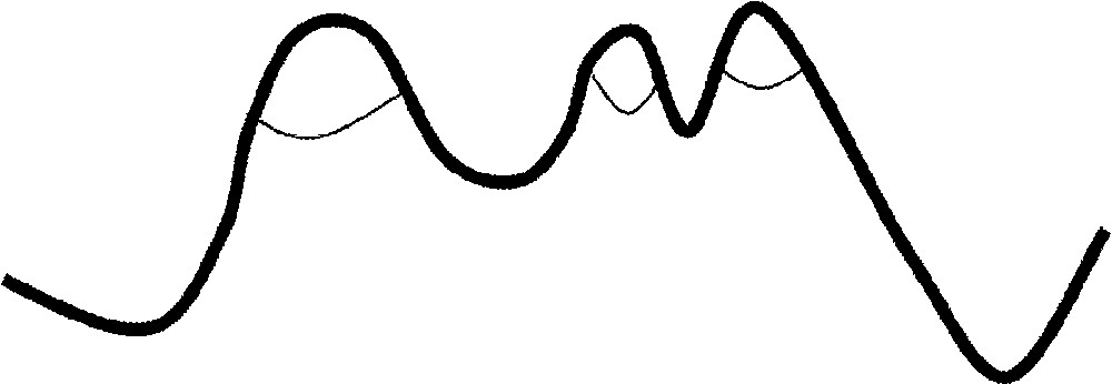
The grey landscape and the characteristic line.
Some types of images (and particularly those previously discussed) are formed of ‘mesas’ or peaks whose shape is close to a Gaussian peak. For such images, we replace all the mesas by their characteristic line. We are thus led to consider the new height function H(x,y) instead of the function g(x,y) and its level line H(x,y) = 0. We display after a plane differential system of which this line is a limit cycle. Let H’(x,y) be the function:
Vanishing of H’(x,y) occurs on the contour line of the maximum of the gradient of g. Consider first the following raw system:
The first term is of steepest descent nature and along this flow, the orbits converge to the zeros of H’(x,y) (Fig. 4). On the set of zeros of H’(x,y), the second Hamiltonian term, which is of convective type, becomes preponderant. Parameters α and β can be used to tune the speed of convergence of the differential system to the limit cycle. To cope with random noise and numeric instabilities, we modify slightly the system into:
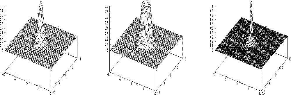
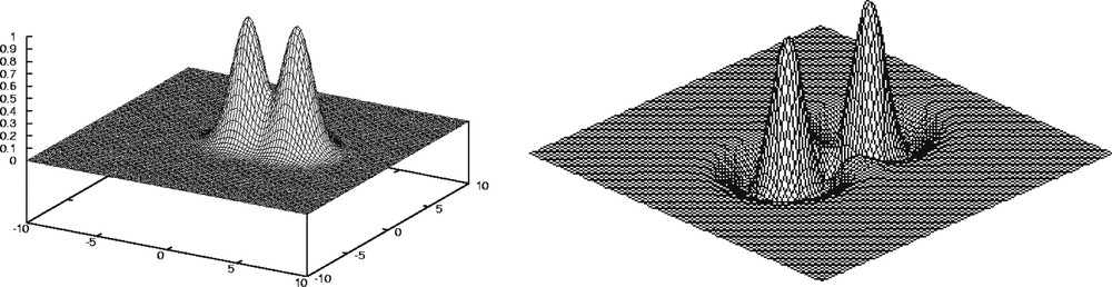
Different peaks for the function g (left), G (centre) and H’ (right).
The added term 〚H(x,y)/G(x,y)〛 speeds up the descent to the vanishing of H(x,y) and forces the stability. The usual discretisation of Runge–Kutta yields ultimately the algorithm, which is quite easy to implement. On each pixel (boundary effects are neglected), the function H(i, j) reads:
An important property of the characteristic line is that in the case of a Gaussian peak, it contours a volume equal to 2/3 of the total volume of the peak (Fig. 5). This property remains exact in case of moderate kurtosis and skewness of the peak. An advantage of our techniques is that we do not perform a direct segmentation of the grey levels of the film.
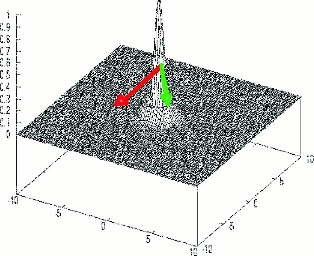
Representation on a peak of the potential (green) and Hamiltonian (red) forces.
Thus the segmentation is much finer than the corresponding one performed in the watershed lines method (or in its variant with markers). We only segment the upper part of the peak and we multiply by 3/2 the activity integrated in the interior of the characteristic line. This approach is interesting, because the lower part of the peak is often noisy. The method seems particularly efficient when the mesas are well separated. If they are close (Fig. 6), then we need to tune parameters α and β.
g (left) and H’ (right) functions for close peaks.
In further developments of the method, we look for an adaptive dynamical calculation of these parameters in terms of the data. If the peaks are not sufficiently separated, the obtained contour corresponds to a domain including the two peaks and the final segmentation is obtained either by tuning the parameters α and β and restarting with the same algorithm, or by manually drawing the inner contours (Fig. 7).
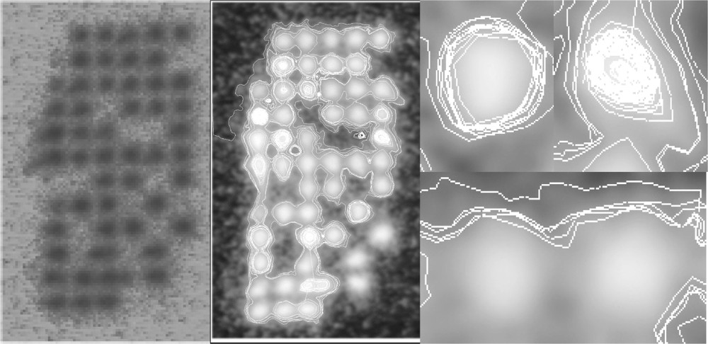
Initial image (left), segmented image (centre) with succeeding trajectories (separated peaks, top right) and failed ones (close peaks, bottom right).
Finally, we affect to each gene a standardised rectangle containing an activity coded through a grey level scale and eventually we reorganise these rectangles in order to detect a co-expression of genes whose proteins are located in same part of the metabolic graph (Fig. 8).
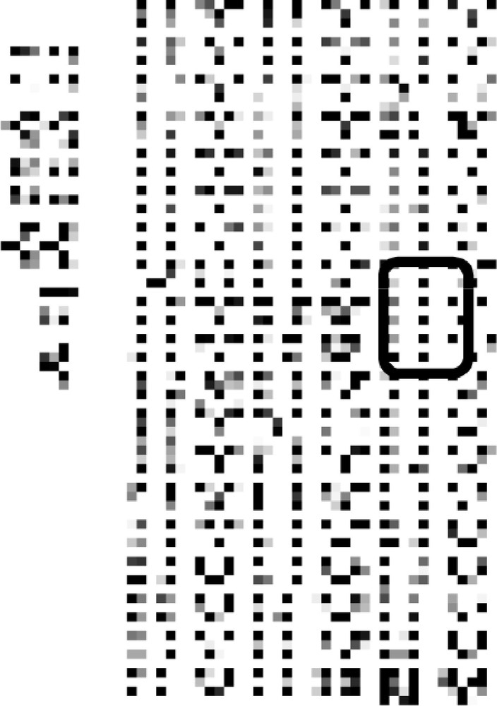
Standardisation of the bio-array image (the black rectangle localises the sub-image treated in Fig. 7 above).
3 Comparison with the watershed method
The watershed line is a concept firstly defined by geographers in order to characterise the main features of a landscape 〚6–11〛: a drop of rain that reaches the ground will flow down to a sea or an ocean. In the case of France, the watershed line splits the country in two parts, the Atlantic zone and the Mediterranean zone. Those zones are called ‘catchment basins’, and the oceans are the minima of them. They define a partition of the relief, and the frontiers of catchment basins define on the pixels plane the watershed line. We can easily understand the interest of this concept in image processing: grey level images can be considered as relief structures, and the watershed line is a good way to separate light (low) zones from dark (high) ones. It is particularly interesting to determine the watershed line of the symmetrical landscape obtained by considering the new grey level 1-g, where g is the initial grey level and if we have taken the maximum of g as a normalised value equal to 1. The watershed line verifies a variational principle: when progressively filling with water a catchment basin, its inner area passes through a series of inflexion points corresponding to the successive saddle points reached by the water. Each inflexion point corresponds to a local maximum of the second derivative of this inner area. The watershed line is computed on discrete image, by immersion simulation, locating the watershed line on the meeting points of several catchment basins. First discrete algorithms of watershed computing by immersion simulation were proposed in 〚7–10〛 for a discrete operator related to the watershed. In our case, the watershed line is computed on the inverse image, in order to have one and only one local maximum (of the original image) into each catchment basin. Then the resulting labelling (still not a partition) is used on the original image. We use the Vincent–Soille algorithm 〚6〛 on discrete images with a linear complexity (about 7.25 N, where N denotes the number of pixels in the image), which can be used in n dimensions.
Figure 9 above shows that the watershed method leads to an over-segmentation of the peaks, in particular when the inner area of the peaks is large. The images obtained in Fig. 7 for isolated peaks prove that this over-segmentation is absent.
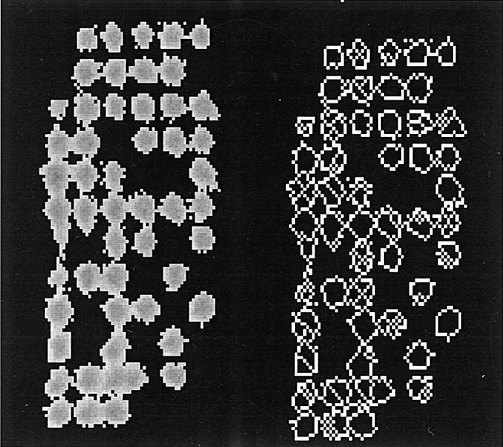
The image of Fig. 7 treated by a watershed method (left) and the corresponding segmentation (right).
4 Conclusion
We have shown in this paper an application of the potential-Hamiltonian segmentation to the bio-array peaks contouring. There are also possible applications for compression of medical images, especially for tele-medical purposes and for matching computer-assisted surgery or for cell tracking in histology 〚12–19〛. This procedure is particularly useful, when one needs rapidly contours for objects of medical interest for helping medical or surgical actions 〚20, 21〛 like brain tumour punctures, cell proliferation studies or fast determinations of large genetic interaction graphs (like those involving several thousands of genes among the 4×10⁴ genes of the human genome), e.g. for counting their positive and negative loops 〚22〛.
Remerciements
We have done this work thanks to the support of the ACI ‘Telemedicine and Technology for Health’ from the French Ministry of Research.
Version abrégée
Les puces à ADN ou bio-arrays produisent des images révélatrices des pics d’activité d’expression des gènes d’une cellule. Ces images ont une structure particulière et l’objet de cette note est de présenter une approche mathématique qui en permet l’analyse automatique. La méthode employée peut être utilisée pour d’autres types d’images présentant des pics d’activité fonctionnelle ou des pics de concentration. L’approche mathématique proposée ici repose sur des techniques élémentaires de géométrie différentielle et de systèmes dynamiques et donne lieu à un algorithme simple, mais efficace, en particulier lorsque les pics sont isolés. Cet algorithme, testé sur des images de bio-arrays fournies par l’équipe de F. Berger (U 318 Inserm), s’est révélée digne d’intérêt par rapport aux autres algorithmes classiques de traitement d’images, comme le gradient seuillé et le calcul de la ligne de partage des eaux (watershed line) : dans ce dernier cas, en particulier, on obtient un sur-contourage des pics, difficile à corriger. Cet article est organisé en trois parties, dans lesquelles sont présentées successivement une description du dispositif expérimental expliquant la nature particulière des images produites par des bio-arrays, puis une présentation de l’algorithme et de ses résultats, enfin, une conclusion et des perspectives de développements futurs.
Depuis quelques années, afin de diagnostiquer certaines maladies, on utilise des appareillages appelés bio-arrays (micro- ou macro-arrays) ou puces à ADN (DNA chips), qui ne diffèrent que par leur échelle d’étude et qui seront désignés dans la suite sous le terme général de bio-arrays.
La mise en application de ces puces repose sur la cartographie du génome et a pour but de quantifier l’expression des gènes que l’on souhaite étudier à un moment donné de la vie cellulaire. Ces bio-arrays fournissent des images qui correspondent à l’intensité d’expression d’un groupe de gènes au moment où la mesure est effectuée.
Il existe deux techniques généralement employées dans les bio-arrays : l’une se fonde sur une analyse de la radioactivité d’isotopes fixés aux ADN simple brin obtenus par transcription inverse à partir des ARN messagers (ARNm) spécifiques des gènes exprimés (Multiplex Messenger Assay), l’autre sur une analyse de fluorescence d’acides nucléiques hybridés marqués (National Human Genome Research Institute). Les deux méthodes diffèrent peu : au lieu d’utiliser des bases radioactives, comme dans le premier cas, on utilise, dans le second cas, des bases nucléiques fluorescentes. Dans les deux cas, on produit les images en utilisant un capteur sensible, soit à la radioactivité, soit à la fluorescence. Dans le second cas, les images produites ont plusieurs canaux de couleurs, mais cela ne conduit à aucune spécificité importante concernant l’algorithme proposé.
La première étape consiste, pour chaque gène à étudier, à sélectionner sa séquence complémentaire, appelée ADNc. Ces ADNc sont reproduits en grande quantité par une opération de réplication de séquences d’ADN (PCR), puis fixés selon un quadrillage du support (plaque de nylon activé, de verre ou de membrane). Sur ce quadrillage, tous les ADNc d’un même gène sont localisés au même endroit sur la plaque. La deuxième étape consiste à extraire les ARNm de la culture de cellules à étudier. Ensuite, on insère ces ARNm dans un milieu où les bases nucléiques A,C,T,G sont substituées par des bases équivalentes, mais radioactives ou fluorescentes, par transcription inverse de l’ARNm de culture. Dans une troisième étape, on place les séquences radioactives ou fluorescentes sur la plaque, où elles se fixent sur les séquences correspondantes d’ADNc. Enfin, on produit l’image à partir de la radioactivité ou de la fluorescence sur la plaque, à l’aide d’un système physique permettant l’amplification et la visualisation (détecteur phosphore, photo-multiplicateur...).
Soit g(x,y) la fonction d’altitude qui, à un pixel de coordonnées (x,y), fait correspondre le niveau de gris de l’image en ce pixel. La ligne caractéristique est définie comme étant l’ensemble des points où la courbure moyenne de Gauss s’annule. Dans le cas d’un pic gaussien isotrope, la ligne caractéristique est une ligne de niveau, et même une ligne de Dupin de gradient constant, mais, en général, le pic n’est pas gaussien, ce qui exige l’usage de méthodes spécifiques de calcul des points qui la composent. Son équation est :
Certaines images (en particulier celles décrites précédemment) sont formées de mesas, ou pics de formes proches de celle d’une gaussienne (à un kurtosis (aplatissement) ou à une skewness (anisotropie) près). Pour de tels pics, on remplace la mesa tout entière par le pic situé au-dessus de sa ligne caractéristique et on multiplie par 3/2 son volume (comme dans le cas d’un pic gaussien pur) pour estimer le volume de la mesa initiale. On est ainsi naturellement amené à considérer la nouvelle fonction d’altitude H(x,y) à la place de la fonction g(x,y) ; il s’agit alors d’en déterminer une ligne de niveau : H(x,y) = 0. Pour ce faire, on va construire un système différentiel du plan qui admet cette ligne comme trajectoire asymptotique. Soit donc H’(x,y) la fonction définie par :
L’annulation de H’(x,y) se fait sur le contour du maximum du gradient de g. Le but est maintenant d’effectuer une segmentation délimitée par le contour représentant le lieu des maxima du gradient de g. On se positionne sur cette ligne en simulant un système différentiel qui admet cette ligne comme cycle limite. Le système différentiel est défini par :
Le premier terme est un terme de descente de potentiel ; cette technique requiert de positionner la condition initiale dans une zone à segmenter, ce qui peut être automatisé en tirant au hasard les données initiales et en supprimant les fichiers des trajectoires suffisamment proches d’un cycle limite déjà obtenu. Lorsqu’on atteint les zéros de H’(x,y), ce terme devient sans influence sur la trajectoire. Le second terme est un terme hamiltonien convectif, qui est un vecteur perpendiculaire au gradient. Les paramètres α et β servent à ajuster la vitesse avec laquelle les trajectoires du système différentiel convergent vers le cycle limite. Afin de supporter le bruit de fond et les incertitudes numériques, on transforme le système (3) en (4) :
Le terme ajouté 〚H(x,y)/G(x,y)〛 oriente la descente vers l’annulation de H(x,y). Le gradient de g tend vers zéro lorsqu’on part vers le centre du pic ou lorsqu’on dépasse la ligne caractéristique. L’inverse de la norme du gradient tend à accentuer la vitesse du système dans ces deux zones, dont il faut qu’on s’éloigne. C’est donc un terme qui force la stabilité. On peut alors développer une discrétisation, qui donne immédiatement lieu à un algorithme facile à implémenter. La fonction H(x,y) se calcule en effet en chaque pixel (on néglige les effets de bord) par :
On peut enfin discrétiser le système différentiel (4) par une méthode de Runge–Kutta de pas ϵ.
Nous l’avons vu, une propriété importante de la ligne caractéristique est que le volume délimité par un « emboutissage » vertical du pic passant par elle est égal aux 2/3 de l’intégrale du pic complet dans le cas Gaussien pur. Cette propriété reste valable en cas de kurtosis (aplatissement) et de skewness (anisotropie) modérés du pic. L’avantage de cette technique est qu’on n’effectue pas une sommation de tous les niveaux de gris d’un pic d’activité (en particulier de ceux se trouvant à la périphérie du pic – souvent très bruitée). La segmentation obtenue est bien plus fine que celle fournie par la méthode de la ligne de partage des eaux (ou sa variante avec marqueurs). On ne segmente que la partie haute du pic, ce qui présente un avantage certain, car la base du pic est bruitée ou superposée à celles des pics voisins. La méthode présentée ci-dessus semble être optimale lorsque les mesas ne sont pas trop rapprochées. Si elles sont trop proches, il faut alors jouer sur les paramètres libres α et β. Des développements futurs de la méthode pourront sans doute conduire à un calcul dynamique optimalisant ces paramètres en fonction des données de l’image. Des développements de l’algorithme sont espérés pour d’autres types d’images médicales, en particulier celles qui nécessitent des méthodes de morphologie mathématique. Les applications possibles concernent autant la compression des images médicales, en vue d’une utilisation en télé-médecine, que l’aide au diagnostic automatique.