

1 Introduction
In their letter to Nature, Courtillot and Gaudemer 〚1〛 show a good fit between a logistic model and biodiversity increase after a mass extinction. Following the authors, data concern historical records of marine (number of families) organisms as a function of geological times compiled by Sepkoski 〚2–4〛 in large databases. They have been compiled to represent variations of the number of families along geological times 〚4〛. Then a question arises: why does a logistical model seem to be well adapted to describe these data? Already Feller 〚5〛 noted that many events in biological dynamics look like a logistic curve and proposed alternative models to describe sigmoid growth curves. Conversely, and more recently, it has been shown that different biological or ecological mechanisms can lead to a logistic model 〚6, 7〛. We discuss a new parameterisation and other formulations of this model, in order to give additional information and suggest a hypothesis about global evolution of biodiversity on a geological time scale. Although the logistic model can be explicitly solved, we worked on its differential expression, which is better adapted to a discussion about elementary mechanisms.
Courtillot and Gaudemer 〚1〛 proposed the following classical expression of the logistic model to describe the changes in number of families during discrete time segments of the last 600 Myr:
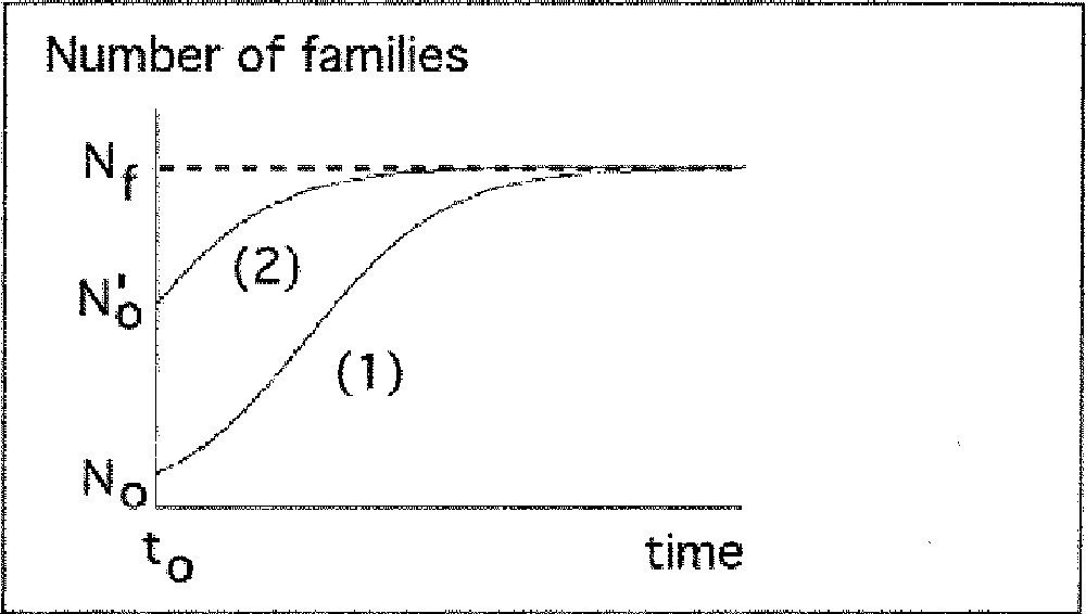
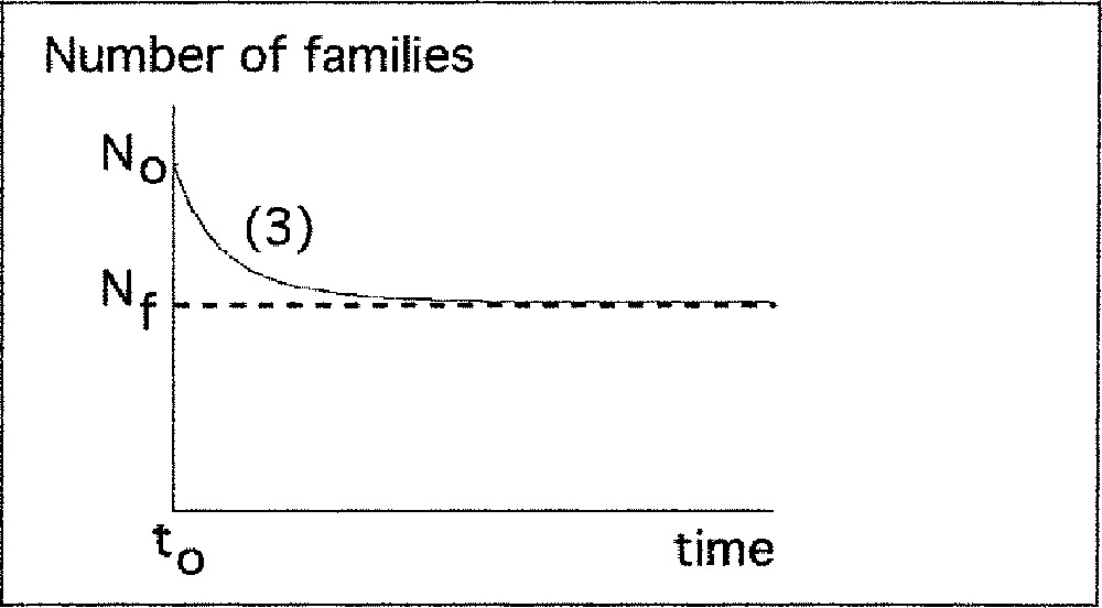
Description of increasing and decreasing phases of biodiversity by the logistic model.
a) Increasing period
The number of families rises during time (N0 < Nf). Nf is the measure of total number of ecological niches.
b) Decreasing period
N0 > Nf : the number of families decreases. It can be interpreted as a loss of ecological niches at time t0, which corresponds to a disappearance of families.
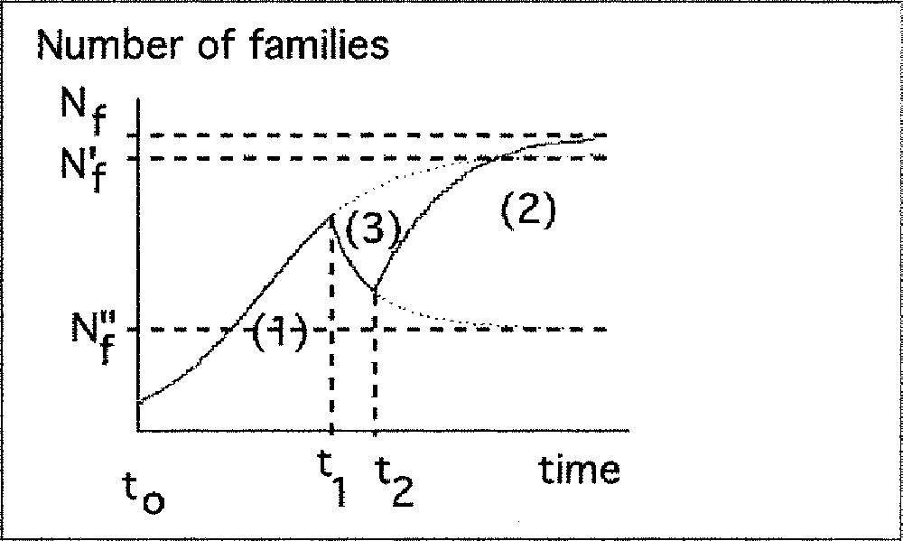
c) Succession of increasing and decreasing periods
Between t0 and t1, the amount of ecological niches is Nf’.
Between t1 and t2, the amount of ecological niches is Nf’’.
After t2, the amount the amount of ecological niches is Nf.
d) Relationship between data and model
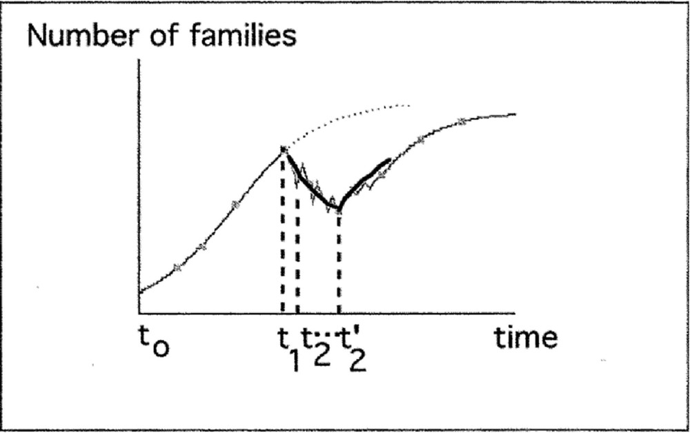
Between t1 and t’2, there is a succession of logistic decreasing (e.g., between t1 and t2) and increasing phases. But data cannot distinguish these phases. Fitting a logistic model gives a global view of the average decreasing number of families during this interval of time. The same remark can be done for an average increasing phase (e.g. just after t’2).
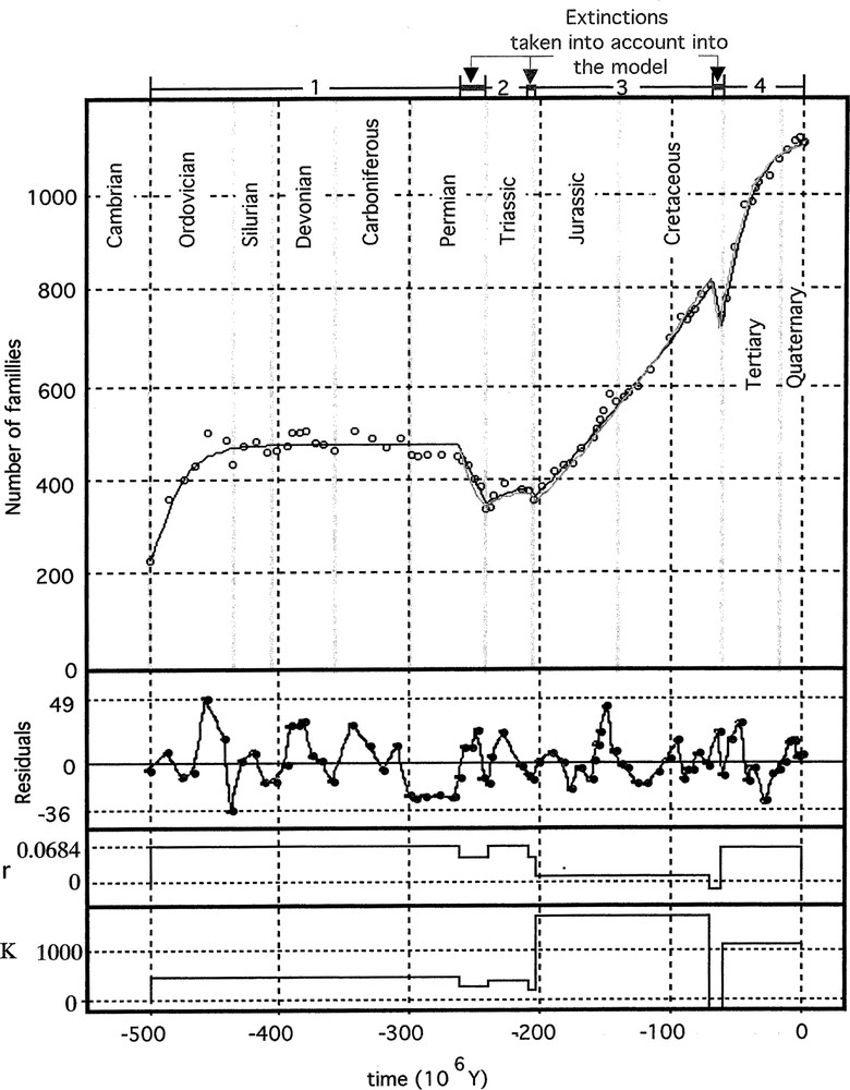
Chained models 〚3〛 and 〚4〛 fitted to data. The increasing number of families is represented by a logistic model, the decreasing one, during a crisis, by an exponential model with a negative exponent (model 〚3〛, dark line) or by a logistic equation (model 〚4〛 or model 〚10〛, light line). Then only the initial condition (N0) at –500 Myr is estimated. The values of r and K of the logistic model are also represented. The residuals give an idea of environmental ‘minor’ perturbations.
- • the values of α are roughly inversely proportional to the relative number of families having disappeared in the previous extinction (the larger the extinction, the greater the biodiversity explosion);
- • an apparent increase in equilibrium level (Nf) after a mass extinction is probably related to a multiplication of ecological niches.
2 Data, method and results
From the same set of data 〚4〛, parameters have been estimated with a similar least squares method. Similar values have been obtained. They are associated to guesses of parameter precisions and correlations. Fig. 3 shows the (α, Nf) plane, and precisions of parameter estimates.
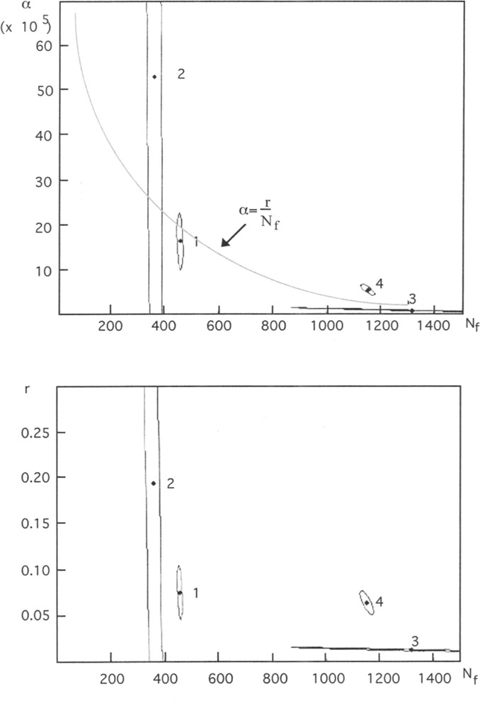
Guesses of parameters α and Nf (model 〚1〛, Fig. 3A), r and and Nf (model 〚2〛, Fig. 3B), and their confidence domains. These graphs show that parameters are correlated, and underlines the low precision of the estimates for the second period. The numbers refer the to following periods: Ordovician to Permian (1), Triassic (2), Jurassic to Cretaceous (3), and Tertiary to Quaternary (4). An ellipse approximates the confidence domain. It corresponds to a linear approximation of the model at the proximity of the minimum of the least-squares criterion 〚7〛. The relation between parameters α, r (introduced in the new parametrisation) and Nf is hyperbolic (Fig. 3A).
In fact, changes in the numbers of niches can be mainly interpreted as corresponding to environmental changes and/or specialisation of species that occupied more and more specific niches and/or sharing of the same niches by several species. This is the question we wish to mainly discuss in this paper.
2.1 New parameterisation of the model and model fitting
In a finite limited environment, the real number of new families is only a part of the potential exponential increase in the number of families: only those that can find a free well suited niche can survive. For a newborn family, the probability to find an occupied niche is, in a first approximation, N/Nf, then the probability to find a free one is 1 – N/Nf. So, the number of really new families becomes:
This other form of logistic model can be formally deduced from (1) if we assume α = r/Nf (cf. Fig. 3A for a graphic interpretation).
If we consider the graph in Fig. 3B, the projections on the r axis (ordinate) are embedded. So, we have tested the following hypothesis: is it possible to consider r as globally constant during all the considered geological interval of time? The model does not fit well (the sum of square is 75 150, to compare to 20 295 – cf. Table 1). However, we tried other possibilities by continuing to apply the principle of parsimony to select models that fit well, with a minimum number of parameters. Among them, the following ones, where the extinction process is also represented, yield good results (cf. Table 1).
Numerical results of non-linear ordinary least squares estimation of parameters. The thrift principle has been applied to obtain a minimum number of estimated parameters. Among all tested possibilities, the chained model 〚3〛 is the best and after the chained model 〚4〛. The value of residual sum of squares (S.Q.) shows that model 〚3〛 fits almost as well as the non-chained model (with four parameters less, this sum only increases of about 5%). When needed in the text, approximate confidence intervals are given. For model 〚1〛, numbers in parentheses refer to Courtillot and Gaudmer’s estimates of α, N0 and Nf.
| Models | Periods | α (× 105) | r (× 102) | N0 estimates | N f | S.Q. |
| Independent models | 1 | 16.2 (15.7) | 7.4 | 203 (204) | 458 (459) | |
| dN/dt = α N (Nf – N) | ||||||
| or | 2 | 53.3 (56.0) | 19.2 | 306 (310) | 360 (364) | |
| dN/dt = r N (1 – N/Nf) | 3 | 0.86 (1.2) | 1.14 | 349 (340) | 1317 (1120) | |
| N0 is estimated after each crisis | ||||||
| (12 estimated parameters, 3 for each period) | 4 | 5.39 (5.31) | 6.22 | 747 (752) | 1153 (1143) | 20 295 |
| Chained model (3) where 8 parameters are estimated: | 1 | 6.87 (± 0.48) | 210 | 459 (± 4) | 21 580 | |
| dN/dt = r N (1 – N/Nf) | ||||||
| (non extinction periods) | 2 | 6.87 (± 0.48) | 364 (± 11) | |||
| dN/dt = –b N | ||||||
| (extinction periods) | ||||||
| N0 is estimated only at the beginning of the first period | 3 | 1.05 (± 0.48) | 1473 (± 278) | |||
| b is the common extinction rate (estimation is 0.0158 ± 0.0016 Myr–1) | 4 | 6.87 (± 0.48) | 1146 (± 11) | |||
| Chained model (4) where 8 parameters are also estimated: | 1 | 6.84 (± 0.54) | 211 | 457 (± 4) | 23 711 | |
| dN/dt = r N (1 – N/Nf) – {b N, during extinction periods, 0 elsewere} | 2 | 6.84 (± 0.54) | 365 (± 11) | |||
| N0 is still estimated only at the beginning of the first period | 3 | 1.01 (± 0.54) | 1610 (± 371) | |||
| b is the common extinction rate (estimation is now 0.0241 ± 0.0026 Myr–1) | 4 | 6.84 (± 0.54) | 1148 (± 11) |
These results suggest, to a first approximation, that r (the inner biological mechanism of differentiation) is globally constant, except during the third period: six times lower than during other periods (the approximate confidence intervals are: 0.0639–0.0735 (model (3)) or 0.0630–0.0738 (model (4)) for periods 1, 2 and 4, and 0.0057–0.0153 (model (3)) or 0.0047–0.0155 (model (4), for period 3). In the next section, we will examine possible interpretations by using the following alternative expressions of the logistic model.
Parameter b represents the apparent time constant of the decreasing processes from data (b = 0.0158 Myr–1). Half of the initial number of families is reached after time T0.5 = (1/b) ln 2, that is to say T = 43.9 Myr. The Cretaceous–Tertiary extinction corresponds to the disappearance of about 9% of families, 91% remains untouched, then the duration of extinction is estimated to be T0.91 = –1/b ln (0.91) ≈ 6 Myr. These values are greater than estimates from chrono-stratigraphic data (about or less than 1 Myr); for example, Olsen et al. evaluate at 0.04 Myr the duration of the extinction period at the end of the Triassic 〚8〛. The discordance between estimations from global model and field chrono-stratigraphic data can be explained: data are too rough to enable precise estimations, so the evaluation of parameter b is common to the three major extinction periods chosen by Courtillot and Gaudemer, whose durations are different; for instance, the Permian–Triassic transition is longer than other ones; it covers, in fact, five successive events, as noted by Hallam and Wignall 〚9〛: three extinctions (whose time is less than 1 My) and two radiations. Data on more recent periods also show a great variability, both in time and amplitude of extinction phenomena (see 〚10〛 on the Palaeogene mammalian record). So b can be interpreted more as a statistical parameter, which permits to link periods and then to obtain a chained model, than a characteristic quantity of extinction processes. In fact, the resolution of data does not allow evaluating such an estimate.
2.2 Other ways to obtain the logistic model and their interpretations
But other forms of the logistical model can also be explored. Among them, if we introduce an additional variable, named for example S, and if N still represents the observed variable, for instance the number of families, the following differential system is another form of this model 〚6〛:
In this context, S can be interpreted as the number of free ecological family niches (a family ecological niche is the set of niches of ecological species which belong to a same family) with the initial conditions N = N0 and S = S0.
The concept of ecological niches is a corner stone in theoretical ecology (a recent presentation can be found in Begon et al. 〚11〛). It was proposed by Hutchinson 〚12〛, and completed after (Vandermeer presented an historical compilation 〚13〛). It can be seen like “an n-dimensional domain of environmental parameters and variables whithin which organisms of a species can maintain a viable population” (adapted from Begon et al., op. cit.). At the beginning, these parameters and variables were physicochemical, then necessary resources were introduced and also other species which can interact with this species are progressively considered as elements of the niche (e.g., competitors, predators). Progressively the concept of niche leads to describe environmental conditions that permit the survival and development of organisms and populations of a species. This concept was first introduced to describe the actual world, from an ecological point of view. But it can be introduced in long term analysis, particularly for the evolution of living systems by introducing environmental changes during the past and responses of living systems to these changes. In such a context, changes of genetic structures, which lead progressively to new species and then to be more or less adapted to environmental changes (i.e. to be able or not to find new niches), has to be considered as dynamics processes. Here we propose to extend the concept of niche, defined for species, to other taxonomic levels, particularly families one. Finally, this concept is global, its concrete realisations are habitats, referenced in space and time. The set of habitats constitute the niche of a taxon.
We have dS/dt = – dN/dt, then S – S0 = – (N – N0) and S = S0 + N0 – N. S and N have the same units; N0 is a measure of occupied niches, S0 is a measure of free niches at t = 0. S(t) represents the amount of free niches at time t (t > 0). Finally, it leads to the logistic model:
In a first approximation, the rate of emergence of new families is proportional to the total number of existing families and to the amount of free niches (S). Newborn families occupy free niches, and then the amount of these niches decreases as they become occupied (formally: S(t → +∞) = 0 and N(t → +∞) = Nf; cf. Fig. 1: increasing period).
But this model does not include a possible spontaneous disappearance of families. Introducing such a mechanism is consistent with actual experimental data on extinction dynamics (see, for example 〚14〛). Now we propose to introduce such a mechanism:
As above, we have dS/dt = –dN/dt, S = S0 + N0 – N or S = k – N, and
This is always the same equation as 〚2〛, with r = (α k – β) and Nf = k – β/α.
If r > 0 and Nf > N0, we observe a growing phase. It is the case for the periods (1), (2), (3), and (4).
If we suppose now that during some periods, called extinction ones, there is in addition a ‘mortality’, consequence of an environmental perturbation as we introduced in model 〚4〛, it also leads to an analogue expression:
Finally, the classical formula, can be proposed to describe all phases:
This formula can describe both the growth parts and decreasing parts of the change of number of families. If r > 0, this is the classical logistic model, K represents the asymptotic equilibrium point, which can be denoted Nf (the final number of families which could occupy the same number of ecological niches). If K = Nf > N0 we observe a growing process from N0 to Nf, and if K = Nf < N0, N decreases from N0 to Nf (cf. Fig. 1: decreasing period). But r can be less than 0 (i.e. r < b) and for the same reason K < 0. In this case, the asymptotic number of families is 0 (the other equilibrium point is – K; obviously, it has no significance). This is an exponentially decreasing process. In practice, and as observed from data, environmental variations and speciation processes (i.e. biological diversification) have avoided reaching such a fatal fate, up to now...
Finally, another way to obtain the logistic model, in this framework, is to consider a constant variation of the number of ecological niches S during an interval of time:
We still have dS/dt = –dN/dt and S = S0 + N0 – N. The parameter u can be positive or negative. Simple calculus leads to the expression: dN/dt = α N (K – N), where K = S0 + N0 + u, if u < 0 then K < N0 + S0 and if u > 0 then K > N0 + S0. So, the logistic model can also take into account constant, positive or negative, additional variations of ecological niches during an interval of time and not only its initial value S0.
Then this model can represent a succession of positive and negative environmental stresses. Practically, one can see the variations of the number of families as a succession of increasing and decreasing phases described by the logistic model, following the values of K and r. These values depends on the ‘mortality’ of families, internal or induced by an environmental perturbations, and of the amount of free niches and its variations, which can also be consequences of such perturbations (Fig. 1: succession of increasing and decreasing periods). No hypothesis is formulated on the size of the interval of time t1 – t2. It can be smaller if the precision of data is sufficient. In fact, as mentioned above, we use data that just enable to evaluate an average process of biodiversity decreasing and increasing on very long intervals of time (e.g., the last case in Fig. 1). It is important to underline that it is a choice to use global data in the goal of analysing a global process, even if there are more precise data. For example, to analyse the variation of the vegetation at the planetary level, we do not use individual data concerning each plant or tree; data are aggregated to represent large biome levels. Here the approach is similar.
3 Discussion and conclusion
Results are summarised in Table 2 and in Fig. 2. As mentioned at the beginning of this article, the discussion turns mainly around the ‘biodiversity explosion’, considering the problem of extinction widely discussed in the literature, and the methodology employed to analyse data.
Parameter values of the logistic model 〚10〛, estimated from expression 〚4〛 (cf. Table 1) or calculated for extinction periods from the common estimate of parameter b. During extinction periods, the previous values of r and Nf are assumed to be the same as those during the preceding growth phase. The negative value of K at the End-Cretaceous has no significance, as explained in the text. In this case, the logistic model looks like an exponential one with 0 as asymptotic value.
| Ordovician–Permian | End-Permian | Beginning-Trias | End-Trias | Jurassic–Cretaceous | End-Cretaceous | Tertiary–Quaternary | |
| r | 0.0684 | 0.0443 | 0.0684 | 0.0443 | 0.0105 | –0.014 | 0.0684 |
| K | 459 | 297 | 365 | 236 | 1610 | –2168 (0) | 1168 |
3.1 Methodological aspects
As already observed by Courtillot and Gaudemer, the logistic model seems to be well adapted to describe global biodiversity changes all along the geologic ages, both on a quantitative basis (it fits well the data) and on a qualitative one (it describes well increasing and decreasing phases). As shown in this article, it can be interpreted in terms of ecological mechanisms, with an explicit introduction of ecological niches. Moreover, the last expressions allow further developments. For example, by introducing in equation (6) a difference in family disappearance and in corresponding ecological niches releasing, we obtain the Kostitzin’s model. System (6) becomes:
However, if this is theoretically satisfying, data do not permit such subtlety (even if we retain equation (6), we can just estimate α K – β and α – K/β).
There is a little difference between the two chained models (3) and (4) whose fitting results are summarised in Table 1. The advantage of the second one is to have a simple representation and to be more satisfying, because there is no evidence that during a global decreasing phase, there is no appearance of new families. The advantage of the first one is to fit better, particularly for the growth phases (3) and (4). However, as shown in Table 2, the differences are globally small and related interpretations are the same.
3.2 Ecological and biological aspects
The surprising fact consists in the importance of diversification, despite drastic environmental perturbations. This diversification is evaluated both by parameters r and K (or Nf).
Since the beginning of the Cretaceous, Nf has increased strongly: from 459 during the first phase and 365 during the growth part of the Triassic, to more than 1000 for the last increasing periods 3 and 4. This can be interpreted in the following different ways: (i) an increase of ecological niches following environmental perturbations (e.g. parcelling out of the environment), and/or (ii) the appearance of new mechanisms of diversifications.
Another explanation (iii) consists in a limitation of growth during period (1), as a consequence of drastic successive perturbations; then, the observed plateau is lower than the one which would have been observed without them, and might be of the same magnitude than for periods 3 and 4.
In the same way, is it possible to propose an explanation for the low value of r during period 3, associated to a very long growth? Does it correspond to an internal biological mechanism that makes lower the rate of diversification (e.g., genetic diversification), or, as suggested by hypothesis (iii) above, to successive perturbations, not sufficient to stop diversification but which curb the increase in the number of families?
In fact, the low value or r (0.0101) compared to the value for other phases (0.0684), can be related to the well known regular ‘minor’ extinctions during this period 〚9, 15, 16〛, which was not sufficient to stop the growth of biodiversity, but which could make it slower.
From data used in this article, a possible evaluation of perturbations can be obtained from the residual sums of squares. They result from sampling errors, from second order variations (e.g., the continuous background of minor extinctions) and from bias introduced by the non-linearity of the model. First, if we examine these variations, the larger ones can be associated to ‘minor’ extinctions, whereas the non-linearity bias can be corrected by calculating the centred sum of squares. Finally, these centred sums of squares (CSQ) correspond to different time intervals, and then it has been weighted by dividing by the durations of periods (RCSQ/Δt (My)). So from models (3) and (4), and only on the growth parts corresponding to phases 1, 3 and 4, excluding the Triassic period (too poor in data), we obtain the results consigned in Table 3.
Simple analysis of residuals: the period (3) is characterised by the lower average variations of observed values around the calculated ones (see text for the definition of the quantity RCSQ/Δt).
| (1) Ordovician–Permian | (3) Jurassic–Cretaceous | (4) Tertiary–Quaternary | ||||
| Periods | Model 〚3〛 | Model 〚4〛 | Model 〚3〛 | Model 〚4〛 | Model 〚3〛 | Model 〚4〛 |
| Residual average | 0.46 | Idem | 1.28 | –3.86 | 1.70 | – 0.99 |
| RCSQ/Δt | 52.2 | Idem | 16.0 | 24.4 | 41.4 | 41.5 |
We can note that the bias introduced by the non-linearity of models and measured by residual averages is very low. This confirms the adequacy of these models to describe data. The ‘sample errors’ are reported on Benton’s graphs 〚4〛, but to ensure the legibility of the graphs they have not been reported in Fig. 2. We just note that after the Devonian, they have more or less the same amplitude than the size of the points. So the oscillations around the curve can mainly be attributed to perturbations.
The values of the residuals by Myr have the same magnitudes for the first and fourth periods, but this value is lower for the third period. In some way, it confirms the hypothesis of a slowing down of the growth during this period, but which is not sufficient to stop the biodiversity increase.
But, even if there are only few data for the fourth period, why is diversification speed so large as compared to the first one, despite the observed perturbations? And why does the apparent number of ecological niches become so large? In fact, if newborn families strictly occupy niches released after extinction, the new plateau would have the same magnitude as the first one. For example, after the Triassic, the biodiversity overshoot this plateau. So, its recovery and overshoot cannot be explained only by the colonisation of released niches, but by the appearance of new niches and/or by ecological mechanisms. After the Triassic, the parcelling out of the super-continent increases the area of coastal zones and consequently the number of marine niches. For instance, the North Atlantic Ocean was formed during the third period and led to coastal zones expansion 〚17〛. But, on the one hand, we have no evidence to consider that the total number of niches is larger than the one in the first period before Pangea, formed in the mid-Palaeozoic. And, on the other hand, we have to explain also the acceleration and the overshoot of the last phase.
Now, let us consider biological and ecological points of view. Among many explanations, we can think of two complementary hypotheses:
- • the first one concerns genetic aspects (the appearance of new genomic mechanisms that favour the emergence of new variants, new species, new genera and new families);
- • the second one is related to the emergence of new ecological relations that could lead to an apparent increase in ecological niches.
If we consider these hypotheses, we can refer to Michod’s work on Darwinian dynamics 〚18〛. Michod proposes that, during geological times, the appearance of cooperative mechanisms between living entities is a major mechanism of evolution. He demonstrates that this hypothesis is consistent with Darwinian theory. So, coexistence and cooperation between macromolecules led to cells, and coexistence and cooperation between cells led to multicellular organisms. He assumes that cooperation appeared progressively and probably sequentially for each level of organisation and therefore allowed the emergence of these levels. Then we may think that what permitted the emergence of cells and organisms could act in the same way at higher levels of organisation, particularly at ecological levels. Even the general tendency is to privilege competition and predation as major mechanisms in ecosystem functioning, it is well known that exist also few mechanisms of coexistence (parasitism) or cooperation (e.g., symbiosis, mutualism). And perhaps we have to re-estimate the relative importance of these mechanisms to explain the functioning of ecosystems and their evolution.
So a similar ecological niche could be shared by different species belonging to different families (no exclusion, but coexistence and/or cooperation). Then biological diversification will proceed not only from multiplication of ecological niches, but also from a kind of ‘niche-sharing’ mechanism resulting from coexistence and cooperation. It may be a way to understand why diversified ecosystems exist today and how they evolved, like present-day intertropical forests, although some ecological mechanisms, such as competition, should lead to simplification (e.g., competitive exclusion). In fact, we can think that scale factors are badly taken into account, particularly spatial ones. Competition is certainly determining at the local scale of the individual tree: it occupies progressively a piece of space during an interval of time (during its life), and therefore limits the possibility to another tree to grow in its immediate neighbouring. Except specific edaphic or climatic conditions, competition is probably less important at higher scales. We can also denote that cooperative processes between species at the root level have been detected (e.g. by the way of mycorrhiza 〚20–22〛).
Moreover, diversification and interactions between elements lead to complex systems, which seem to make them more resilient. It is a hypothesis widely shared by ecologists to promote the interest of diversified systems. Although it is not completely demonstrated at this level of organisation, it has been shown recently that a network of interrelated (cooperative) elements allows large variations of parameters, without significant consequences on the systems (for example, cf. von Dassow et al.’s work on a gene network of Drosophila m. 〚19〛). Then cooperative mechanisms, and resilience of ecosystems, as a consequence of interrelations between organisms, are in favour of diversification, at least in the long term.
In this framework, it is reasonable to assume that cooperative and evolutive mechanisms at the molecular and cellular levels have been stabilised for a rather long time (e.g. for the cellular level, since the first multicellular radiation), and that ecological ones are probably more recent and would explain large diversification, as a consequence of appearance of ecological niche-sharing during the last period (and perhaps already during the third one). Perhaps they are always in an evolution phase, not yet stabilised.
So, in a first approximation, we can propose the following scheme of biodiversity increase: molecular processes are more or less established for a long time, then the rate of diversification, estimated by parameter r, is more or less constant (the low value during the third period could be the consequence of successive minor extinctions). But to survive and to be observed in natural archives, a new taxon needs to be ecologically stabilised during a sufficient time. Then the observed increase of biodiversity should result from new ecological relationships, such as coexistence and cooperation, which favour niche-sharing and then ecological stabilisation and the increase of the apparent number of niches (parameter K).
However, we cannot exclude the emergence of new processes at the genomic level, such as transposon moving or virus integration, and we must not forget, in the end, that differences between taxa are expressed at the genomic level, whichever the involved mechanisms. Then diversification could be seen as a progressive adaptation between genomic dynamics and the emergence of new ecological relations (e.g., co-evolution). This enhances the interest of coupling researches between these two ‘distant’ levels: the molecular one and the ecological one.
At the molecular level, it would be of great benefit to find at which time genomic mechanisms of diversification appeared. Are they old, as suggested by Michod, or more recent? Searching pieces of sequences that look like moving parts of genomes, dating them, and testing if the incorporation process is homogeneous during the envisaged period (from Cambrian to actual) could help, through the study of known DNA sequences, to test this assumed consequence of Michod’s hypothesis.
At the ecological level, an exciting topic of research should be to make an effort in palaeoecology. The concept of niche is related to spatial distribution. So, one of the main problems is to reconstruct spatial distributions of organisms and populations in palaeoecosystems and the evolution of these structures, in order to verify the progressive appearance of niche-sharing, and then to assume the correlated appearance of coexistence and cooperative mechanisms. Conversely, if such relationships are not still stabilised, which is very plausible, we may have the opportunity to observe an evolutionary mechanism in action. In fact, more and more studies on ecological interactions, called ‘long-term interactions’, such as host-parasite ones, already go in this direction (cf., for example, 〚23〛). This leads one to ask whether present actions of Man, which results in new kinds of perturbations on ecosystems, could disturb the existing relationships, or stop the natural emergence of new ones, and then lead to the ‘Third Mass Extinction’, following P. Ward 〚24〛, or the ‘sixth extinction’ feared by Leakey and Lewin 〚25〛.
Version abrégée
V. Courtillot et Y. Gaudemer 〚1〛 ont proposé d’utiliser le modèle logistique pour représenter les variations de la biodiversité à l'échelle géologique, caractérisées par le nombre de familles. Ils se sont focalisés sur les phases de croissance, sachant que les phases de décroissance ont été largement étudiées par ailleurs. Aussi, ces auteurs ont-ils ajusté ce modèle pour différentes périodes en particulier, (1) du début de l’Ordovicien au début du Permien, (2) la phase croissante du Trias, (3) le Jurassique–Crétacé et (4) le Tertiaire–Quaternaire. Nous avons adopté le même point de vue, en poursuivant leur analyse, notamment en proposant diverses interprétations du modèle logistique dans ce contexte. Ainsi, la paramétrisation, dite r,K, classiquement adoptée en écologie, peut être utilisée. Le paramètre r représente le taux intrinsèque de variation de la biodiversité, le paramètre K les potentialités du milieu en termes de niches écologiques. De plus, pour minimiser le nombre de paramètre à estimer, nous avons construit deux modèles chaînés prenant en compte les phases de décroissance, soit par un modèle exponentiel, soit par un modèle logistique. Il apparaît que la valeur du paramètre r peut être considérée comme identique pour les périodes (1), (2) et (4), mais qu’elle apparaît significativement plus petite pour la période (3). Le paramètre K, représentant le plateau, est significativement plus élevé pour les périodes (3) et (4) que pour les précédentes. Durant la troisième période, le plateau n’est pas atteint, la crise Crétacé–Tertiaire interrompant le processus. Mais celui-ci reprend rapidement pendant la période Tertiaire–Quaternaire, avec la même valeur de r que pour les périodes (1) et (2).
Une autre formulation de ce modèle permet de faire entrer explicitement le nombre de niches écologique comme variable d’état ; on montre alors comment on peut retrouver simplement les expressions précédentes. L’avantage de cette formulation est qu’elle permet des développements ultérieurs et une meilleure interprétation des mécanismes sous-jacents.
L’augmentation de la biodiversité pourrait être interprétée comme une conséquence :
- • de la création de niches écologique à la suite de perturbations environnementales ;
- • de l’apparition de mécanismes nouveaux au niveau génétique ;
- • de l’émergence de nouvelles relations écologiques.
D’une part, on peut raisonnablement supposer que les perturbations environnementales détruisent autant, sinon plus, de niches écologiques qu’elles n’en créent, et que, même en imaginant un processus de restauration, ces perturbations se sont produites de façon « régulières » dans le temps et ne suffisent pas à expliquer les explosions de la biodiversité. D’autre part, en reprenant l’analyse de Michod 〚18〛 sur la dynamique darwinienne, on est amené à penser que les mécanismes génétiques (au niveau moléculaire), y compris de diversification, ont été probablement stabilisés avant l’apparition des premiers métazoaires. Sans pour autant oublier que les différences entre taxons correspondent fondamentalement à des différences entre génomes. Ainsi, l’apparition d’organismes multicellulaires correspondrait à la mise en place de processus de coopération entre cellules, les cellules étant apparues précédemment grâce à l’émergence de processus de coopération entre macromolécules. Si on émet l’hypothèse que ces processus de coopération, probablement précédés par la coexistence, se mettent en place progressivement et successivement pour tous les niveaux d’organisation du vivant jusqu’à l’écosystème, on peut penser que cela conduirait plusieurs espèces, genres et familles, à pouvoir occuper la même niche écologique et donc entraînerait une multiplication apparente de ces niches. Nous proposons ainsi que des mécanismes de coexistence et de coopération au niveau écologique, qui n’étaient que peu présents dans les périodes précédentes (r « normal » et K faible) se sont mis en place dans la période « récente» Tertiaire–Quaternaire (r « normal » et K élevé), peut-être – et dans une moindre mesure – dès la période Jurassique–Crétacé (r faible et K élevé).
Ainsi, le schéma évolutif serait le suivant : les processus de diversification génétique, dont le paramètre r exprimerait le taux, seraient en place depuis l’émergence des formes actuelles, à savoir depuis le Cambrien. L’émergence, plus récente, de nouvelles relations écologiques permettrait une stabilisation des nouveaux taxons suffisamment longue pour qu’ils puissent être observables dans les archives paléontologiques. La mise en place de ces nouvelles relations (coexistence et coopération) expliquerait l’augmentation apparente du nombre de niches écologiques durant les deux dernières périodes (K élevé). La faible valeur de r durant le Jurassique–Crétacé serait alors interprétée comme l’effet d’une succession de perturbations environnementales conduisant à des extinctions « mineures ».