Modelling individual plant growth at a variable mean density or at a specific spatial setting

Christian Damgaard

doi:10.1016/j.crvi.2003.05.001

Biological modelling / Biomodélisation

Modelling individual plant growth at a variable mean density or at a specific spatial setting

Présenté par : Pierre Auger

Christian Damgaard ¹

¹ Department of Terrestrial Ecology, DMU, Vejlsøvej 25, 8600 Silkeborg, Denmark

Comptes Rendus. Biologies, Volume 327 (2004) no. 3, pp. 255-260.

Résumé

Neighbouring plants generally compete for the limiting resources in order to grow and reproduce. Some resources, e.g., sun light, may be monopolised by the larger plants and this may lead to asymmetric competition where a plant, which is twice as large, grows more than twice as fast. A previously published individual-based Richards growth model that describes the asymmetric growth of individual plants is here generalised with respect to a variable mean plant density and an explicit spatial setting.

Métadonnées

Reçu le : 2003-04-15
Accepté le : 2003-05-25
Publié le : 2004-03-01

PMID

DOI : 10.1016/j.crvi.2003.05.001

Mots clés : size-asymmetric competition, Richards growth model, plant growth, individual-based modelling

Affiliations des auteurs :

Christian Damgaard ¹

¹ Department of Terrestrial Ecology, DMU, Vejlsøvej 25, 8600 Silkeborg, Denmark

@article{CRBIOL_2004__327_3_255_0,
     author = {Christian Damgaard},
     title = {Modelling individual plant growth at a variable mean density or at a specific spatial setting},
     journal = {Comptes Rendus. Biologies},
     pages = {255--260},
     publisher = {Elsevier},
     volume = {327},
     number = {3},
     year = {2004},
     doi = {10.1016/j.crvi.2003.05.001},
     language = {en},
}

TY  - JOUR
AU  - Christian Damgaard
TI  - Modelling individual plant growth at a variable mean density or at a specific spatial setting
JO  - Comptes Rendus. Biologies
PY  - 2004
SP  - 255
EP  - 260
VL  - 327
IS  - 3
PB  - Elsevier
DO  - 10.1016/j.crvi.2003.05.001
LA  - en
ID  - CRBIOL_2004__327_3_255_0
ER  -

%0 Journal Article
%A Christian Damgaard
%T Modelling individual plant growth at a variable mean density or at a specific spatial setting
%J Comptes Rendus. Biologies
%D 2004
%P 255-260
%V 327
%N 3
%I Elsevier
%R 10.1016/j.crvi.2003.05.001
%G en
%F CRBIOL_2004__327_3_255_0

Christian Damgaard. Modelling individual plant growth at a variable mean density or at a specific spatial setting. Comptes Rendus. Biologies, Volume 327 (2004) no. 3, pp. 255-260. doi : 10.1016/j.crvi.2003.05.001. https://comptes-rendus.academie-sciences.fr/biologies/articles/10.1016/j.crvi.2003.05.001/

Version originale du texte intégral

1 Introduction

Neighbouring plants generally compete for the limiting resources and, in order to understand the effect of neighbouring plants, it is essential to compare and test different hypotheses of the effect of neighbours. It is possible to test many simple hypotheses using informal and verbal models, but verbal models may be susceptible to vagueness and logical pitfalls, especially if the model is complicated. On the other hand, by constructing a mathematical model, which encapsulates the hypothesis that we want to test, we are forced to be precise in the description of the functional relationships.

Two fundamentally different approaches can be made when modelling plant growth.

(1) The expected effects of the abiotic and biotic environment, including effects of neighbouring plants, on plant growth may be modelled using mechanistic plant models. In a mechanistic plant model [1–4], the growth rate of different plant species is modelled as a function of the limiting resource(s). Such mechanistic plant models ideally contain detailed information of how plants respond to different environments, which enables predictions of plant growth as a function of the environment. In reality, the models necessarily contain many more or less alleged functional relationships and many parameters that are difficult or impossible to estimate jointly.
(2) A less ambitious approach, which will be followed here, is to describe plant growth using empirical models that are fitted to plant growth data. Empirical models are mathematically simple models with relatively few biologically interpretable parameters, and due to their simplicity it is possible to jointly estimate all the parameters in the model from a single dataset. The joint estimation of parameters is important if there is any covariability between parameters. The empirical models rely heavily on data and the model will never be better than the underlying data; thus, it is important to be conscious of the limitations of empirical models, e.g., it is not possible to make predictions outside the domain of the data. Since plant growth data typically has been obtained at a fixed environment, empirical models have been criticised for having limited predictive power; however, this limitation may be circumvented by obtaining ecological data along an environmental gradient. In constructing empirical plant growth models, there is a delicate balance between keeping models simple and describing the biological system in sufficient detail to obtain the desired information, i.e., performing tests of investigated hypotheses or obtaining posterior distributions of biological parameters.

2 Richards growth model

Several sigmoidal or saturated growth models have been proposed to describe growth of individual plants, e.g., Gompertz, and logistic growth models where the main difference between the models is when the plant experiences its maximum growth rate [5]. The maximum growth rate occurs at the point when the sigmoidal growth curve shifts from being convex to being concave (the inflection point) and, in the Richards growth model [6], this inflection point is modelled by a free parameter. The determination of the inflection point by a free parameter makes the Richards growth model relatively flexible and inclusive of the other sigmoidal growth models (Fig. 1). Rather than assuming a fixed point of inflection, the Richards growth model is assumed in the following, since there is no general theory that predicts at what growth stage plants experience their maximum growth rate, and the inflection point has been shown to depend on density [7].

Fig. 1
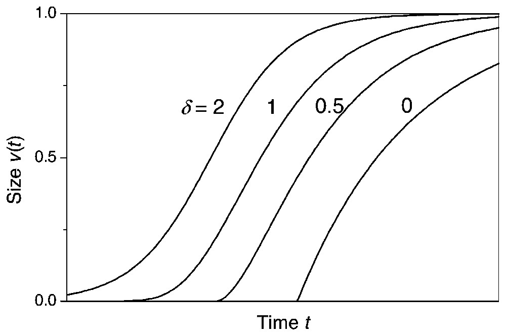
Curves of Richards growth model for various δ, w=1 and κ is 0.75, 0.5, 0.375 and 0.25, respectively. The parameter γ is changed each time so that the curves do not sit on top of one another. The variable inflection point controlled by the parameter δ makes the Richards growth model inclusive of the other sigmoidal growth functions, e.g., the logistic model (δ=2), the Gompertz model (δ=1), and the monomolecular model (δ=0). From [6].

Individual plant growth will in the following be measured by the absolute growth rate, which is the increase in some measure of plant size, e.g., biomass, per time. In the Richards growth model the growth of a plant at time t, is assumed to be proportional to the plant size at time t multiplied by a saturating function of the plant size at time t.

\frac{d v (t)}{d t} = \frac{κ}{1 - δ} v (t) ({(\frac{v (t)}{w})}^{δ - 1} - 1), δ \neq 1

(1)

where v(t) is the plant size at time t, κ is a growth parameter, and w is the final plant size. The initial growth rate is κ/(δ−1) and if δ>1 the initial growth is exponential. The shape of the growth curve is mainly determined by δ. If δ>0, then the growth curve is sigmoidal and the point of inflection is at the proportion δ^1/(1−δ) of the final size. The slope of the tangent at the point of inflection decreases with δ. The plant experiences the maximum growth rate,

κ \underset{\cdot}{w} δ^{δ / (1 - δ)}

, at the inflection point. The saturating term is analogous with the competition term in the logistic model of population growth of individuals towards a carrying capacity [8].

The variable inflection point of the Richards growth model includes other sigmoidal growth functions as special cases (Fig. 1) [5], i.e., the monomolecular model (δ=0), the von Bertalanffy model (δ=2/3), the logistic model (δ=2), and by taking the limit as δ→1 the Gompertz model:

\frac{d v (t)}{d t} = κ v (t) (\log w - \log v (t))

(2)

The Richards growth differential equation may be solved under the condition that for δ<1, (1−δ)×exp(κγ)⩽1 [5]:

v (t) = w {(1 + (δ - 1) \exp (- κ (t - γ)))}^{1 / (1 - δ)}

(3)

where γ is the time of the inflection point.

3 Size-asymmetric growth

The Richards growth model (1) adequately describes the growth of a single plant or plant growth in a monoculture of identical plants. However, the plants in a monoculture are rarely identical. There may be variation in the time of germination, distance to nearest neighbour, or in the microenvironment that leads to variable plant sizes. If the plant growth is limited by a resource that may be monopolised, e.g., light, then asymmetric competition may occur and the variation among plant sizes may increase with time more than expected under a Richards growth model [7,9–12].

In the Richards growth model, the growth of a plant is assumed to be proportional to the plant size multiplied by a saturating function. In order to allow for size-asymmetric growth, the assumption of proportional growth may be generalised so that the growth of plants is proportional to a power function of their size [7,13–15]:

f (v (t), a) = {\begin{matrix} 1, & a = 0 \\ v {(t)}^{a}, & a > 0 \\ 1 or 0, & a = \infty \end{matrix}

(4)

where the effect of plant size on growth is summarised by a size-asymmetry parameter, a, which measures the degree of curvature of the size-growth relationship over the entire growth curve and takes values between 0 and ∞ (Table 1, Fig. 2).

	Parameter value	Definition
Complete symmetry	a=0	All plants have the same growth rate irrespective of their size
Partial size-symmetry	0<a<1	The growth rate is less than proportional to the size of the plant
Perfect size-symmetry	a=1	The growth rate is proportional to the size of the plant
Partial size-asymmetry	a>1	The growth rate is more than proportional to the size
Complete size-asymmetry	a=∞	Limiting case where only a few dominating plants are growing; all other plants have stopped growing

Fig. 2
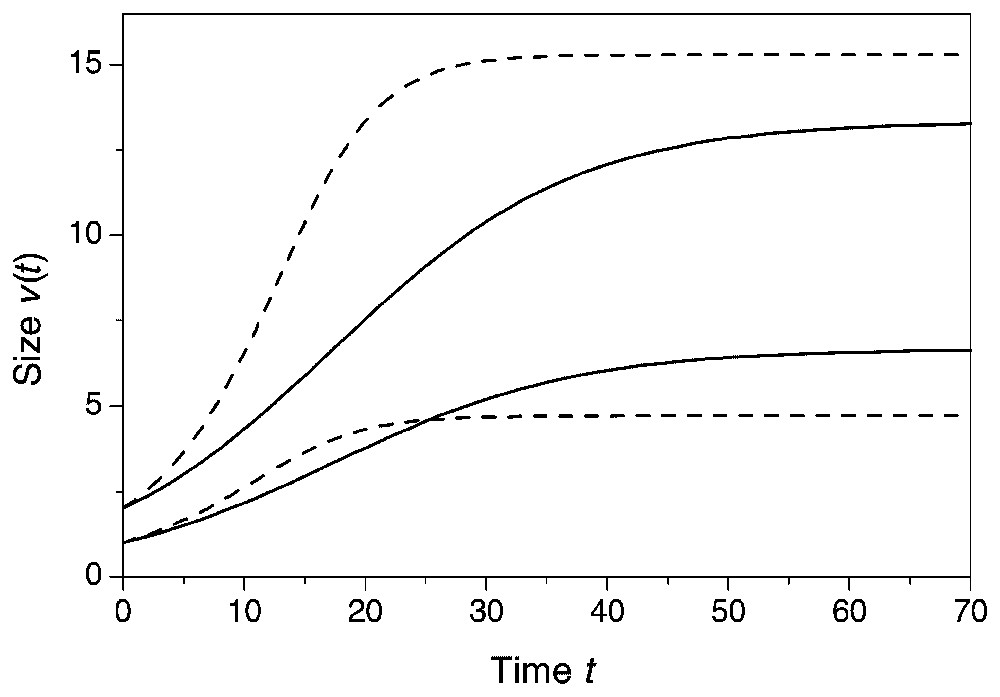
Richards growth model for two interacting plants with and initial size of one and two, respectively at two levels of the degree of size-asymmetry. Full line: a=1, w=10, κ=0.1, δ=2. Dashed line: a=1.5, w=10, κ=0.0667, δ=2. Notice that the size difference increases with a.

In order to take the effect of plant size variation on the growth of individual plants into account, an individual-based Richards growth model may be formulated by generalising (1) and (2) with respect to size-asymmetric growth (4). Assume a monoculture of n competitively interacting plants of variable size, then the growth of plant i at time t may be expressed by n coupled differential equations:

\frac{d v_{i} (t)}{d t} = {\begin{matrix} \frac{κ}{1 - δ} f (v_{i} (t), a) ({(\frac{1}{nw} \sum_{j = 1}^{n} v_{j} (t))}^{δ - 1} \\ - 1), δ \neq 1 \\ κ f (v_{i} (t), a) (\log (nw) \\ - \log (\sum_{j = 1}^{n} v_{j} (t))), δ = 1 \end{matrix}

(5)

[7], where v_i(t) is the size of plant i at time t, and w is the average plant size at the end of the growing season. The initial growth rate is (κa)/(δ−1), and the saturating term

({(\frac{1}{nw} \sum_{j = 1}^{n} v_{j} (t))}^{δ - 1} - 1)

or (log(nw)−log(∑_j=1ⁿv_j(t))), if δ=0, measures the decrease in individual plant growth due to the size and competitive effects of the n interacting plants. The saturation term, which is equal for all n plants at a given time, reduces as the plants grow and when ∑_j=1ⁿv_j(t)=nw the saturation term equals zero and growth stops (Fig. 2).

The individual-based Richards growth model cannot be solved in the general case, and in order to fit the growth model to growth data, the model has to be solved numerically for each set of parameter values used in a maximum-likelihood fitting procedure [7].

4 Effect of plant density

In a number of empirical studies (e.g., [17–20]) the class of hyperbolic size-density response functions has been demonstrated to fit plant competition data well at different growth stages and for different measures of plant size. [21] introduced a hyperbolic size-density response function for a single species:

v (x) = {(α + β x^{ϕ})}^{- 1 / θ}, α, β > 0

(6)

where x is the density of plants or number of plants in a unit area. The shape parameters φ and θ make the response function quite flexible, but only two cases are biologically relevant [5,22]. If φ=θ=1, the cumulative size of plants per unit area, xv(x), increases asymptotically with x towards β⁻¹. If θ<φ, the cumulative size of plants per unit area increases towards an optimum at (αθ/β(φ−θ))^1/φ after which the cumulative size decrease. Generally, at low plant density (x→0) and for φ>0, v=α^−1/θ. The Bleasdale–Nelder model (6) may be derived from the Richards growth model (1) by assuming an allometric relationship between the size and density, vx^ρ=c, where c is a constant and θ=δ−1,

ϕ = (δ - 1) ρ

[5].

It has been found that it is primarily the ratio θ/φ in the Bleasdale–Nelder model (6) that determines the shape of the plant size-density curve [5,22]. Therefore, a simpler model has been proposed [23,24]:

v (x) = \frac{v_{m}}{1 + β x^{ϕ}}

(7)

where θ in (6) is set to 1. In this simpler model, the shape parameters are easier to interpret biologically. v_m(≈α⁻¹) is the size of isolated plants (i.e., for x→0), β is a measure of competition, including its intensity and the area within which it operates, while φ is a measure of the rate at which competition decays as a function of distance between plants [24].

The individual-based Richards growth model (5) may be extended to include growth at different densities by generalising the four parameters in the individual-based growth model (5) to functions of density. It is apparent that the average final size, w in (5), may be generalised by a plant size-density model, e.g., (7), w(x)=w_m/(1+βx^φ), and assuming that the initial growth rate is independent of density, (κa)/(δ−1)=c, then κ may be generalised to κ(x)=c(δ(x)−1)/a(x), where c is a constant. The functions δ(x) and a(x) may be expected to be decreasing and increasing functions of density, respectively, and likely candidate functions may be δ(x)=δ₀exp(−δ₁x) and a(x)=a₀+a₁x. Generalising the individual-based Richards growth model (5) with respect to density requires at least four new free parameters, thus the fitting and especially the testing of biological hypotheses will require very good plant growth data and has not been done yet.

5 Modelling spatial effects

The plant size-density models (6) and (7) are mean-field models [25,26], where it is assumed implicitly that all individuals at a certain density have the same size, and every plant has the same effect of any other plant. The mean-field approach is a sensible place to begin in the modelling of plant–plant interactions [27], but it ignores much of what is important about the dynamics of plant communities [25]. In reality, interactions typically are restricted to a subset of the individuals as and the likelihood that two plants will interact is most probably a decreasing function of the distance between them [28].

As explained above, the negative interactions between neighbouring plants are caused by competition for the same resources. The ways the limiting resources are distributed among the neighbouring plants depend on the type of resource that is limiting for growth, the interacting plant species and their size. Different theoretical models, which describe the distribution of resources, have been proposed. However, the development of theory in this area has been more rapid than the compilation of relevant ecological data and it is difficult to assess the validity of the different models.

The ‘zone of influence’ model is a resource-uptake-based model, which allows for differences in plant size [29–32]. Each plant is assumed surrounded by an imaginary circle, which symbolises the area from which the plant may extract resources. When the plant grows, the radius of the circle expands according to some species-specific rules. After a while, the imaginary circles of two neighbouring plants may overlap and the resources in the overlapping area are shared among the plants according to species-specific rules of sharing resources. For example, the largest plant may get all the resources in the overlapping area (complete size-asymmetric competition), or plants may share the resources in the overlapping area proportionally to their size (perfect size-symmetric competition). The ‘zone of influence’ model may be generalised by assuming that the influence of the plant within the zone is a decreasing function of the distance from the plant [33].

An empirical spatial model called the neighbourhood model assumes that a plant only competes with the neighbours that are positioned within a fitted fixed radius of the plant [34,35]. The competitive effect of the neighbours and the plant itself (self-shading) on the growth of the plant is described by a mean-field plant size-density model. The neighbourhood model has the advantage that it is readily fitted to data [36]. However, in a comparative test between different spatial models on natural populations of Lasallia pustulata [37], the neighbourhood model (number of plants within a circle with fixed radius) was a worse predictor than the distance to the nearest neighbour, which is also a conceptually simpler model.

Using the distances between plants and a given functional relationship that describes the effect of interplant distances on the competitive interactions, U, such a competitive neighbourhood function may be used to generalise the individual-based Richards growth models (5) with respect to the spatial setting:

\frac{d v_{i} (t)}{d t} = {\begin{matrix} \frac{κ}{1 - δ} f (v_{i} (t), a) \\ \times ({(\frac{1}{w_{m}} \sum_{j = 1}^{n} v_{j} (t) U (λ, r (i, j)))}^{δ - 1} \\ - 1), δ \neq 1 \\ κ f (v_{i} (t), a) (\log (w_{m}) \\ - \log (\sum_{j = 1}^{n} v_{j} (t) U (λ, r (i, j)))) \\ δ = 1 \end{matrix}

(8)

Since the competitive interactions only takes place on a local scale, the terms ∑_j=1ⁿv_j(t) and nw in the saturating terms in (5) is replaced by ∑_j=1ⁿv_j(t)U(λ,r(i,j)) and w_m, respectively, where w_m is the final size of an isolated plant. The competitive neighbourhood function is a two-dimensional density function that describes the negative effect of plant j on plant i as a function of the distance between the two plants, r(i,j), where λ is a scale parameter of the effect of distance. The competitive neighbourhood function is analogous to a competition kernel [38], except that, since local growth is saturated by the final size of an isolated plant, the ‘spatial effect’ of self-shading is defined as being equal to 1. One of the likely candidate functions that describe the effect of interplant distances on the competitive effect is the two-dimensional exponential density function [39]; thus, a candidate competitive-neighbourhood function may be:

U (λ, r (i, j)) = \exp (- λ r (i, j))

(9)

The fitting of such a spatial explicit individual-based Richards growth model (8) requires growth data of individual plants with a known spatial position; the growth model will probably be valuable in the analysis of tree growth, where spatially explicit long-term growth data exist (e.g., [40]).

Acknowledgements

Thanks to Jacob Weiner for inspiring discussions and two anonymous reviewers for fruitful suggestions.

Bibliographie

[1] D. Tilman Dynamics and Structure of Plant Communities, Princeton University Press, Princeton, NJ, 1988

[2] D.H. Deutschman; S.A. Levin; C. Devine; L.A. Buttel Scaling from trees to forests: analysis of a complex simulation model, Science Online, Volume 277 (1997) http://www.sciencemag.org/feature/data/deutschman/index.htm

[3] S. Pacala; C. Canham; J. Saponara; J. Silander; R. Kobe; E. Ribbens Forest models defined by field measurements: estimation, error analysis and dynamics, Ecol. Monogr., Volume 66 (1996), pp. 1-44

[4] Land-Use Changes in European Ecosystems: ECOMONT – Concepts and Results (A. Cernusca; U. Tappeiner; N. Bayfield, eds.), Blackwell Wissenshafts-Verlag, Berlin, 1999

[5] G.A.F. Seber; C.J. Wild Nonlinear Regression, Wiley, New York, 1989

[6] F.J. Richards A flexible growth function for empirical use, J. Exp. Bot., Volume 10 (1959), pp. 290-300

[7] C. Damgaard; J. Weiner; H. Nagashima Modelling individual growth and competition in plant populations: growth curves of Chenopodium album at two densities, J. Ecol., Volume 90 (2002), pp. 666-671

[8] J.H. Verhulst Notice sur la loi que la population suit dans son accroissement, Correspondance Math. Phys., Volume 10 (1838), pp. 113-121

[9] J. Weiner Asymmetric competition in plant populations, Trends Ecol. Evol., Volume 5 (1990), pp. 360-364

[10] J. Weiner Size hierarchies in experimental populations of annual plants, Ecology, Volume 66 (1985), pp. 743-752

[11] J. Weiner; S.C. Thomas Size variability and competition in plant monocultures, Oikos, Volume 47 (1986), pp. 211-222

[12] J. Weiner How competition for light and nutrients affects size variability in Ipomoea tricolor populations, Ecology, Volume 67 (1986), pp. 1425-1427

[13] C. Damgaard A test of asymmetric competition in plant monocultures using the maximum likelihood function of a simple growth model, Ecol. Model., Volume 116 (1999), pp. 285-292

[14] S. Schwinning; G.A. Fox Population dynamic consequences of competitive symmetry in annual plants, Oikos, Volume 72 (1995), pp. 422-432

[15] T. Wyszomirski; I. Wyszomirska; I. Jarzyna Simple mechanisms of size distributions dynamics in crowded and uncrowded virtual monocultures, Ecol. Model., Volume 115 (1999), pp. 253-273

[16] S. Schwinning; J. Weiner Mechanisms determining the degree of size asymmetry in competition among plants, Oecologia, Volume 113 (1998), pp. 447-455

[17] R. Law; A.R. Watkinson Response-surface analysis of two species competition: an experiment on Phleum arenarium and Vulpia fasciculata., J. Ecol., Volume 75 (1987), pp. 871-886

[18] R. Cousens Aspects of the design and interpretation of competition experiments, Weed Technol., Volume 5 (1991), pp. 664-673

[19] K. Shinozaki; T. Kira Intraspecific competition among higher plants. VII. Logistic theory of the C–D effect, J. Inst. Polytech., Osaka City University, Volume 7 (1956), pp. 35-72

[20] C. Damgaard Plant competition experiments: testing hypotheses and estimating the probability of coexistence, Ecology, Volume 79 (1998), pp. 1760-1767

[21] J.K.A. Bleasdale; J.A. Nelder Plant populations and crop yield, Nature, Volume 188 (1960), p. 342

[22] R. Mead Plant density and crop yield, Appl. Stat., Volume 19 (1970), pp. 64-81

[23] A.R. Watkinson Density-dependence in single species populations of plants, J. Theor. Biol., Volume 83 (1980), pp. 345-357

[24] J. Vandermeer Plant competition and the yield–density relationship, J. Theor. Biol., Volume 109 (1984), pp. 393-399

[25] S.A. Levin; S.W. Pacala Theories of simplification and scaling of spatially distributed processes (D. Tilman; P. Kareiva, eds.), Spatial Ecology, Princeton University Press, Princeton, NJ, 1997, pp. 271-295

[26] R. Durrett; S. Levin The importance of being discrete (and spatial), Theor. Popul. Biol., Volume 46 (1994), pp. 363-394

[27] B.M. Bolker; D.H. Deutschman; G. Hartvigsen; D.L. Smith Individual-based modelling: what is the difference?, Trends Ecol. Evol., Volume 12 (1997), p. 111

[28] P. Stoll; J. Weiner A neighborhood view of interactions among individual plants (U. Dieckmann; R. Law; J.A.J. Metz, eds.), The Geometry of Ecological Interactions, Cambridge University Press, Cambridge, 2000, pp. 11-27

[29] T. Hara; T. Wyszomirski Competitive asymmetry reduces spatial effects on size-structure dynamics in plant populations, Ann. Bot., Volume 73 (1994), pp. 173-190

[30] D.J. Gates; M. Westcott Zone of influence models for competition in plantations, Adv. Appl. Probab., Volume 10 (1978), pp. 299-537

[31] J. Weiner; P. Stoll; H. Muller-Landau; A. Jasentuliyana The effects of density, spatial pattern and competitive symmetry on size variation in simulated plant populations, Am. Nat., Volume 158 (2001), pp. 438-450

[32] T. Wyszomirski A simulation model of the growth of competing individuals of a plant population, Ekol. Pol., Volume 31 (1983), pp. 73-92

[33] U. Berger; H. Hildenbrandt A new approach to spatially explicit modelling of forest dynamics: spacing, ageing and neighbourhood competition of mangrove trees, Ecol. Model., Volume 132 (2000), pp. 287-302

[34] S.W. Pacala; J.A. Silander Neighbourhood models of plant population dynamics. I. Single species models of annuals, Am. Nat., Volume 125 (1985), pp. 385-411

[35] D.A. Coomes; M. Rees; L. Turnbull; S. Ratcliffe On the mechanisms of coexistence among annual-plant species, using neighbourhood techniques and simulation models, Plant Ecol., Volume 163 (2002), pp. 23-38

[36] S.W. Pacala; J.A. Silander Field tests of neighborhood population dynamic models of two annual species, Ecol. Monogr., Volume 60 (1990), pp. 113-134

[37] N. Sletvold; G. Hestmark A comparative test of the predictive power of neighbourhood models in natural populations of Lasillia pustulata, Can. J. Bot., Volume 77 (1999), pp. 1655-1661

[38] B.M. Bolker; S.W. Pacala; S.A. Levin Moment methods for ecological processes in continuous space (U. Dieckmann; R. Law; J.A.J. Metz, eds.), The Geometry of Ecological Interactions: Simplifying Spatial Complexity, Cambridge University Press, Cambridge, 2000, pp. 388-411

[39] The Geometry of Ecological Interactions: Simplifying Spatial Complexity (U. Dieckmann; R. Law; J.A.J. Metz, eds.), Cambridge University Press, Cambridge, 2000

[40] P. Soares; M. Tomé Distance-dependent competition measures for eucalyptus plantations in Portugal, Ann. For. Sci., Volume 56 (1999), pp. 307-319

Commentaires - Politique