

1 Introduction
During the recent years, the rapid development of the bio-arrays techniques [1] based on isotopic or fluorescent activity of hybridised DNA chips allowed the biologist to give to a grey level peak the signification of an expression rate for the genes studied in the bio-array. If we repeat this acquisition at different times of the cell cycle for different cells of a same tissue, we can calculate correlations between the genes expression rate and hence we are able to make explicit a matrix W called the intergenic interaction matrix, representing the repression and induction influences a gene can exert on other genes.
1.1 The raw data from the bio-array imaging
The first encountered problem with the bio-array image is the noise and we have to low-pass it in order to suppress the high-frequency noise (see Fig. 1). The result of this pre-treatment is a better separation of the isotopic activity peaks, allowing a watershed separation and contouring [2,3]. We can also apply a more accurate segmentation and contouring method called potential-Hamiltonian or ‘Gaussian-stamping’ method. Let us remark that the peaks are about Gaussian, with a weak kurtosis and skewness, allowing in particular the respect of the conservation ‘law’: 2/3 of the activity peak are concentrated into the set of points (x,y) where the Gaussian curvature C(x,y) vanishes, i.e. inside the maximum gradient line, called the characteristic line of the peak. Then it is possible to neglect the part of the peak outside the projection of this line, whose equation is C(x,y)=∂2g/∂x2∂2g/∂y2−(∂2g/∂x∂y)2=0, g(x,y) denoting the grey level function at the pixel of coordinates (x,y).
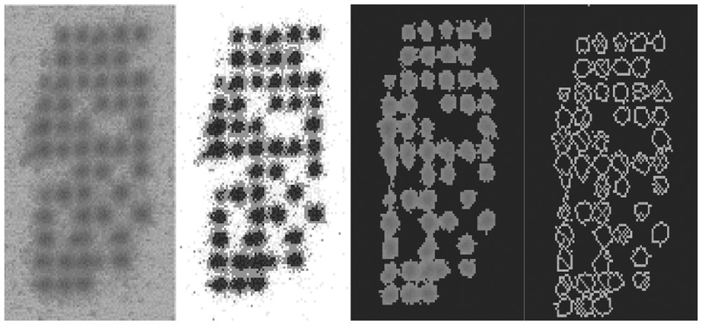
(a) Raw data; (b) low-pass filtering; (c) watershed segmenting; (d) contouring.
We are thus led to consider the new height function C(x,y) instead of the function g(x,y) and its level line C(x,y)=0. A new algorithm has been proposed in [1] to obtain automatically the characteristic line and, after, by integrating inside the projection of this line on the (x,y) plane and multiplying by 3/2 the obtained result, to standardize the estimated activity in terms of a bio-image with small squares symbolizing in grey levels the degree of hybridisation of the cDNA's expressing the regulation of a glioma tissue (Fig. 2). From such bio-array images acquired in cells of the same tissue at different times of the cell cycle, we can study the interactions between genes by estimating an interaction matrix.
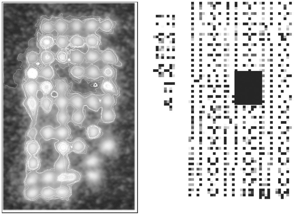
‘Gaussian-stamping’ contours (left) and standardized bio-array image (black rectangle right corresponds to the left image).
2 Some rigorous results about the network attractors
2.1 The interaction matrix
The interaction matrix W is similar to the synaptic weight matrix, which rules the relationships between neurons in a neural network. The general coefficient wik of such an interaction matrix W is equal to +1 (resp −1, 0) if the gene Gk activates (resp inhibits, does not influence) the gene Gi, the state xi of the gene Gi being equal to +1 (resp −1), if it is (resp is not) expressed. In the case of small regulatory genetic systems (called operons), the knowledge of such a matrix W permits to make explicit all possible stationary behaviours of the organisms having the corresponding genome. The change of state of gene Gi between t and t+1 obeys a threshold rule: xi(t+1)=H(∑k=1,nwikxk(t)−bi) or , where H is the sign step function (H(y)=1, if y⩾0 and H(y)=−1, if y<0) and the bis are threshold values. When t is increasing, the genes states reach a stable set of configurations (a fixed configuration or a cycle of configurations), called attractor of the genetic network dynamics. For example, in the regulatory network that regulates the Arabidopsis thaliana flower morphogenesis, the interaction matrix is a (11,11)-matrix with only 22 non-zero coefficients (see Fig. 3). This matrix presents positive loops and attractors (see Section 3.1). Hence it is in general of a great biological interest and relevance to determine matrices having characteristic properties like (i) a minimal number of non-zero coefficients for a given set of attractors (fixed points or cycles) or (ii) a minimal number of positive loops, controlling the number of attractors and their stability (cf. [4–9] for the continuous case [10–12] and for the discrete one). In the following, we intend to partly solve the problems taken above by giving necessary and sufficient conditions to obtain properties (i) and (ii). In order to calculate the wiks, we can either determine the s-directional correlation ρik(s) between the state vector {xk(t−s)}t∈C of gene j at time t−s and the state vector {xi(t)}t∈C of gene i at time t, t varying during the cell cycle C of length M=|C| and corresponding to observation times of the bio-array images:
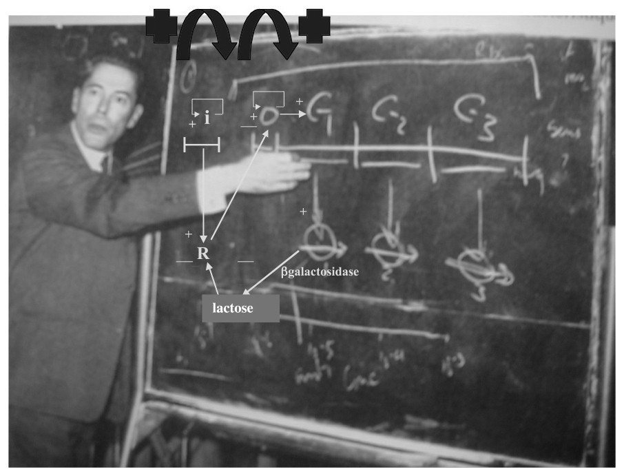
The lactose operon exhibited by Jacques Monod.
If G is the interaction graph associated to W, then we call connected component C of G each set of genes C such that there is a path between every pair of genes of C along a sequence of arcs of G. A Garden of Eden is a gene receiving no arc, but influencing at least one other gene. A regulon is a connected component of G having exactly one positive (auto-catalysis) and one negative loop, these loops sharing the auto-catalysed node. In the lactose operon (see its G in Fig. 3), , , , (βgal-activated and inactivated states), and G has one connected component and one regulon.
2.2 Some definitions and notations
In the following, we give some definitions about the rigorous mathematical description of the discrete Boolean networks used to describe the genes interaction dynamics, and their associated graph G and matrix W. Then we will present some theoretical results with rigorous proofs only for the first and last results in order to show what kind of reasoning we have to perform and we will refer to [13–16] for complete demonstrations. Let us consider a graph G=(V, E), where V={1,…,n} is the set of nodes and E is the set of arcs. Let be a real (n,n)-matrix. We call G the incidence graph of W, if (k,i), the arc going from k to i, belongs to E, then wik≠0. By extension, W will also be called the incidence matrix of G. We will define the sign of an arc (k,i), denoted by sign((k,i)), as the sign of wik. Let us denote by Γ−(i) (resp Γ+(i)) the set of nodes {i1,i2,…,ik(i)} such that (ij,i) (resp (i,ij)) belongs to E, for each j=1,…,k(i). We will say that a set of arcs C={e1,e2,…,er} is a chain if each ek in C has a node belonging to ek−1 and the other one belonging to ek+1. We will say that C is a simple (resp elementary) chain if the arcs (resp nodes) are different. In the sequel we will understand by chain a simple and elementary chain. In the same way we will call C a path if ek=(ik,ik+1) implies ek+1=(ik+1,ik+2), for all k=1,…,r, that is to say the final node of each arc is the beginning node of the next arc in C. The sign of a path or a chain C (denoted by sign(C)) is positive if the number of negative arcs of C is even and negative if this number is odd. A cycle (resp circuit or loop) is defined as a chain (resp path) where each of the two extremities of any arc belongs to two and only two arcs. For simplicity of notation, we will say that a node i belongs to a cycle C if there exists a node j such that (i,j) or (j,i) belongs to C. Every other definition of graph theory used here will be consistent with that in [17,18]. We will call a circuit or cycle C negative (resp positive) if sign(C) is negative (resp positive). Define now a discrete state regulatory network, acting on the set of states {−1,1}, here and subsequently denoted by N, as the 4-uple N=(G, W, b, sign), where G is the incidence graph of W, b is a threshold real vector and the local transition function is given by xi(t+1)=sign(∑k=1,…,nwikxk(t)−bi), , where sign(u)=1 if u⩾0 and sign(u)=−1 otherwise. The sequential iteration consists to update the nodes one by one in a prescribed periodic update I=(i(1),i(2),…,i(n)), where {i(1),i(2),…,i(n)}={1,2,…,n}, that is to say, starting with a given in {−1,1}n, we generate a sequence of iterates:
2.3 Relations between positive and negative cycles, and fixed points
In the sequel, we will assume that the graph G is connected, since otherwise one can apply the results to each of connected components of G. In addition, we will suppose with no loss of generality that |Γ−(i)|>0, for all i∈V. Since otherwise, if there exists a node i∈V such that Γ−(i) is empty, then we can assume that the arc (i,i) exists in E; in this way the dynamics of both networks are the same. It evidently follows from this property that there exists at least one circuit C in G (possibly a circuit of the form (i,i)). Finally, we suppose that the graph G and the matrix W have a quasi-minimal structure, that is to say, all (j,i), such as i≠j, belong to E (or equivalently wij≠0, if i≠j), if there exists , such that:
The following property will be very useful in the following for characterizing a cycle. A cycle C is positive if and only if there exists a vector such that for all (k,i)∈C, sign(wik)=xixk or equivalently, for all (k,i)∈C, .Proposition 1
Let C be a positive cycle and i(0) a fixed node belonging to C. Let us enumerate the nodes belonging to C by i(0),i(1),…,i(j), such that or (i(k),i(k−1))∈C (by identifying j and −1). Finally, let us define the vector x as follows: Proof
Obviously x is satisfying equation (1). Hence –x satisfies equation (1) too. Finally, it is direct that there does not exist another vector that satisfies equation (1).
Let C be now a negative cycle, and let us suppose that equation (1) is true, then ∏(j,i)∈Csign(wij)=∏jxj∏ixi=(∏jxj)2, but sign(C)=∏(j,i)∈Csign(wij)<0, which is contradictory.□
Given N, if all cycles of the incidence graph G are positive, then there exists a vector such that and are fixed points of N.
Theorem 1
There are two remarkable fixed points having by construction a non-frustration property, that is on each cycle the sign changes of xis are identical to the sign changes of the arcs. For other possible fixed points, there is at least one cycle for which sign changes are frustrated.Remark
If all circuits of the incidence graph G are negative, then N has no fixed points.
Theorem 2
2.4 Minimal regulatory networks
The previous results allow us to characterize some minimal regulatory networks. The following propositions constitute examples of minimal regulatory networks. They solve in part the inverse problem consisting in the description of W only from the knowledge of a phenotypic x observed from bio-array images. Let N having n nodes and n connections, a necessary and sufficient condition of existence of a fixed point is the existence of a positive circuit. In this case, and are both fixed points. Hence we can characterize the set of minimal Ns having as fixed point.Proposition 2
Given a state vector , the set of minimal networks having as fixed point is given by the following conditions:Proposition 3
Let N with n nodes and n+1 connections, a necessary and sufficient condition for existence of an attractor of all points parallel iterated, is a negative circuit and a positive circuit intersecting.
Proposition 4
2.5 Fixed points bounds in regulatory networks
Given N, let C be a positive circuit of N, then by Proposition 1, there exists , such that x and −x satisfy the equation: ∀(k,i)∈C, sign(wik)=xixk. We denote u(C)∈{−1,1}|V(C)| the vector defined by: u(C) (resp −x), if xi(0)=1 (resp −1), where i(0)=min{i∣i∈C}. Given N and a fixed vector of N, then for all i∈V, there exists a positive circuit C(i) in G such that for all k in C(i),yk=u(C(i))k or for all k in C(i),yk=−u(C(i))k. If m is the total number of positive circuits of N, then the number of fixed points of N is⩽2m, and this upper bound is reached if and only if for all circuits C of N there does not exist an arc (k,i) in CC ending in C (there is no garden of Eden k pending to C).Lemma 1
Theorem 3
We have to notice that the condition concerns the number of circuits and not of cycles, these last being in general very more numerous.Remark
2.6 Asymptotic mean value for the number of fixed configurations (fixed vectors or limit cycles of vectors) in the case K
Let us consider now a network N having n nodes and 2n connections such as . We search for a mean value of the number of fixed configurations, when n is growing to infinity. For any graph G having m non-oriented edges, the mean number of oriented edges we can define on G from the non-oriented configuration is equal to 4m/3.Lemma 2
Let us note 〈o〉 the mean number of oriented edges we can construct from a configuration of m non-oriented edges; then, if exactly k from the m non-oriented edges are decomposed into two oriented opposite connections, we have Cmm−k2m−k different ways to dispatch the not double connections into the (m−k) other non-oriented edges; hence we can write: .□Proof
If the network N has n nodes and n connections, with , then the expectation of the number of fixed configurations of N is n1/2, if n is sufficiently large.
Theorem 4
Following [19], if the connections of N are random, and if the mean number c of non-oriented edges per node is equal to 3/2, then the random variables Xi equal to the number of disjoint cycles of length i of N are independent and Poissonnian with parameter λ(i)=2i−1/i, if n is sufficiently large. From Lemma 2, we are just in this case, because we have 2n=4m/3 connections, hence m=3n/2 and c=m/n=3/2. Then we have, for the mean number 〈f〉 of fixed configurations of N: , where , ∑i=1ns(i)=s, ∑i=1nis(i)=k}, Πσ=P({Xi=s(i),s(i)⩾0,∑i=1ns(i)=s, ∑i=1nis(i)=k})=e−∑λ(i)∏i=1nλ(i)s(i)/s(i)! is the probability to have the Xis equal each to s(i), and A(σ) is the mean number of fixed configurations, when each Xis is equal to s(i). We will now evaluate the expectation A(σ). Each disjoint positive circuit bringing two fixed points (Theorem 3 above), an isolated positive non-circuit cycle bringing also two fixed points and an isolated negative circuit bringing one limit cycle, we can first calculate A(0,σ), the expected number of fixed configurations in the case where we have only disjoint positive circuits, the rest of the nodes depending on these circuits (and hence their states being fixed by the states of the circuit): A(0,σ)=B(0,σ)/D(σ), where B(0,σ)=2s (number of fixed points of s=∑i=1ns(i) disjoint positive circuits, from Theorem 3 above)×2k (number of different signs for each of the k=∑i=1nis(i)⩽n nodes involved in the s circuits)×[2s (number of different directions – left or right – for each of the s circuits)/2s (reduction factor for having only positive circuits)]×N(σ),D(σ)=2k (number of different directions for each of the k connections)×2k (number of different signs for each of the k connections)×N(σ), where N(σ) is the number of choices for the s disjoint cycles: N(σ)=Cks(1)1,…,s(n)n∏i=1n(i−1)!s(i)/2s. N(σ) just equals the number of choices of k nodes in s(1) subsets of size 1,…,s(n) of size n times the number of choices of different loops (without multiple points) connecting the vertices inside each of these subsets. In the same way, we can calculate A(1,σ) (resp A(j,σ)) the expected number of attractors of N in the case where we have among the s disjoint cycles 1 (resp j) isolated positive non-circuit cycles (bringing two fixed vectors) or isolated negative circuits (bringing 1 fixed cycle). We have also: Proof
where
where s(i)212i2i/21 is just the number (21) of fixed points of 1 positive cycle (circuit or not) of length i times the number of such configurations s(i)(2i2i/21), s(i)2i21/21 is the number (1) of attractors of 1 isolated negative circuit of length i times the number of such configurations s(i) (2i21/21) and −s(i)212i21/21 is the number (21) of fixed points of 1 positive circuit (already counted in B(0,σ)) times the number of such configurations s(i) (2i21/21); 2s−1 (2s−1/2s−1)N(σ)2k−i is equal to the number of configurations of s−1 positive circuits with s(1) of length 1,…,s(i)−1 of length i,…,s(n) of length n. Then we have: A(2,σ)=B(2,σ)/D(σ), where
where s(i)s(j)(222i+j2i+j−(222i+j2i22−212i+j2i22)−(222i+j2j22−212i+j2j22)+2i+j22)/22 is just the number of the fixed configurations of a couple made of positive not circuit cycles or negative circuits, the (s−2) remaining cycles being positive circuits, by paying attention to the fact that the fixed configurations of the couple of a positive not circuit cycle combined with a positive circuit (s(i)s(j)222i+j(2i+2j)22) have been already counted both in B(1,σ) and in B(0,σ) and hence have to be taken away (by using sign−) from the sum s(i)s(j)(222i+j2i+j+212i+j2i21+212i+j2j21+2i+j22)/22.
Finally, more generally, we have A(j,σ)=B(j,σ)/D(σ), where
By summing the A(j,σ)s and after the A(σ)Πσs, 〈f〉 is clearly of the order of n1/2:
Then we have: .□
Remark
3 Examples of genetic regulation networks
3.1 The flowering regulatory network of Arabidopsis thaliana
If we consider the interaction graph of the flowering regulatory network of Arabidopsis thaliana (Fig. 4, right) [10], then we can easily define from it a Boolean dynamics, Fig. 4 (left) giving an example of attractor with final states (in bold red) different from the initial conditions. The characteristics of the associated interaction matrix W are: , , , (corresponding to the 4 differentiated tissues of the flower, i.e. sepals, petals, stamens and carpels). W has two connected components and four gardens of Eden. A(W) is well ⩽24 and in fact exactly equal to 22, where 2 is the number of connected components having at least one positive loop. Then we can recall that:
- – in 1948, Delbrück [21] conjectured that positive loops in the interaction graph of a regulatory network was a necessary condition for cell differentiation, i.e. for the existence of multiple attractors of the genes expression; this conjecture has been written in a good mathematical context by Thomas in 1980 [22]; we have proved above that the positive loops were related to the observation of multiple attractors, which definitively gives to the positive loops another signification than to the negative ones, more related to the stability of the system (like in the classical Watt regulator, well known in cybernetics, cf. Fig. 5);
- – in 1992, Kauffman [20] conjectured that the mean number of attractors for a Boolean genetic network with n genes and with connectivity 2 was of the order of √n (see Theorem 4 above). This conjecture is now supported by real observations: we have about 35 000 genes in the human genome and about 200 different tissues, which can be considered as different attractors of the same dynamics. For Arabidopsis thaliana, there is different tissues [10] and for the Cro operon of the phage , , (lytic and lysogenic attractors) [23,24], with Boolean [25] or discrete multi-level [26] models.
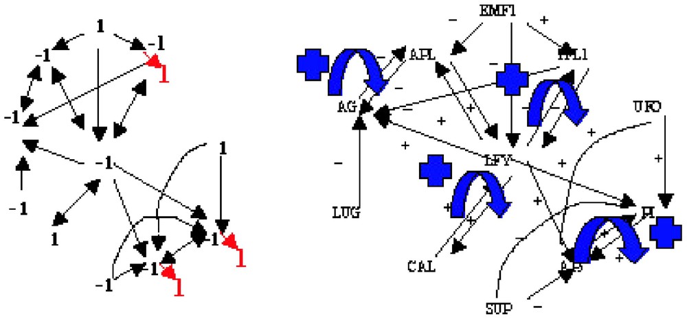
Interaction graph of the flowering regulatory network of Arabidopsis thaliana (right) and an attractor of its Boolean dynamics (left).

The Watt regulator, the prototype of negative regulatory loop in cybernetics.
3.2 The gastrulation regulatory network
If we consider the regulatory network ruling the gastrulation in Drosophila (cf. Fig. 6 and [28]), it is easy to check that , , and (the corresponding cells being the ordinary ectoderm cell and the trapezoidal invagination cell called bottle cell). The regulation graph contains five connected components (among which three are singletons). In this case, the classical Kolmogorov–Rashevski–Turing models of reaction–diffusion [29–31] are well explaining the epigenetic part of the invagination at the start of the gastrulation, but only after the apparition of a new bottle cell presenting an apical constriction due to the change of intracellular balances ATP/ADP and GTP/GDP (whose ratios increase), due to the expression of the kinase (ADK and GDK) genes. This is due to a change of attractor basin by the bottle cell starting the gastrulation process due to the genetic regulation pathway of Fig. 6. This context describing the morphogenesis from genetic and epigenetic forces was called by Waddington a chreode or a morphogenetic landscape (cf. Fig. 7).
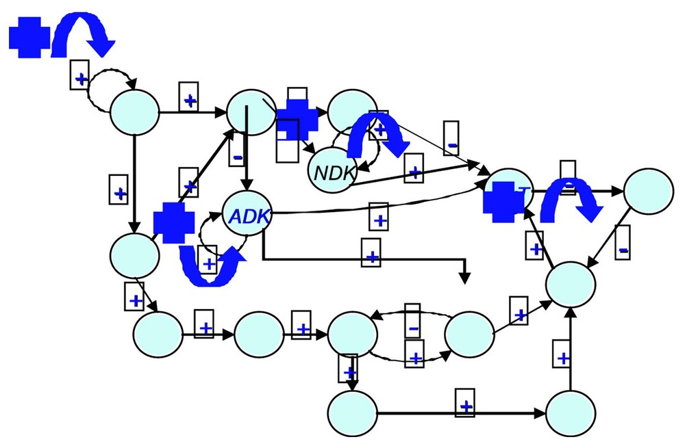
The gastrulation regulatory network (after [27]) (ADK and NDK are respectively the adenylate kinase and the nucleotide diphosphate kinase).
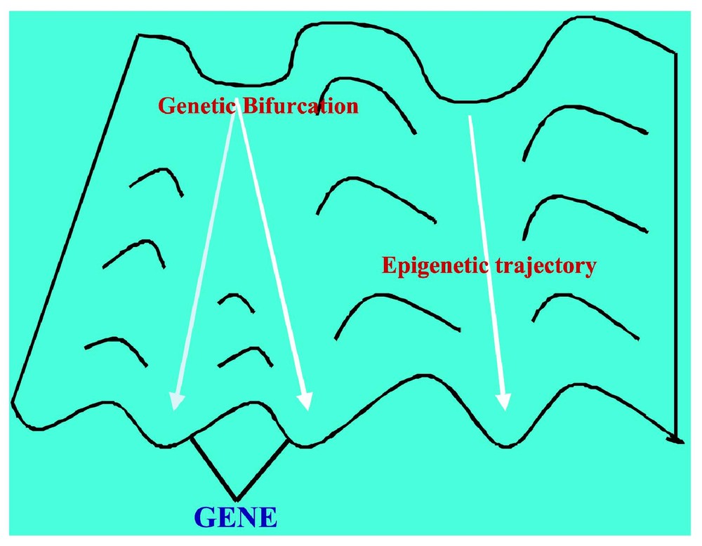
The Waddington chreode or morphogenetic landscape.
3.3 The phage μ lytic-lysogenic attractor [32]
If we consider the operon governing the expression of the phage μ, we obtain the graph given in Fig. 8. It is interesting to notice that , , , (the two corresponding states in the host cell being the lytic and lysogenic ones, like for the Cro operon of the phage λ [24]). There is only one connected component.
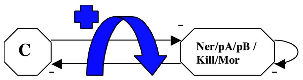
The phage μ operon.
3.4 The mnesic ‘opernet’
We will call in the following mnesic ‘opernet’ the system obtained by merging the genetic (operon) and epigenetic parts (metabolic net) of the system ruling the cotyledonary buds growth (cf. [33,34] and Fig. 9).
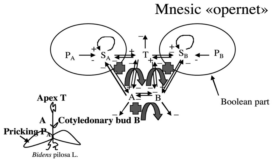
The mnesic opernet.
The genetic part of the mnesic opernet has been modelled by a Boolean system [34]:
- – variable PA (resp PB) represents pricking treatment (or any other stress action) on the side A (resp B) of the plant and its value is 1 if treatment has been done, and 0 if not;
- – variable SA (resp SB) represents the discrete part of the operon; we suppose that it contributes to mobilize a morphogenetic cotyledonary material RA (resp RB) responsible for the growth of the apex and of the cotyledonary bud A (resp B).
We will suppose in the following that the variable RA (resp RB) representing the concentration of R on side A (resp B) is continuous and that its velocity dRA/dt (resp dRB/dt) is ruled by a differential system containing a three-switch between the continuous variables T (apex growth metabolites concentration), A and B (cotyledonary buds A and B growth metabolites concentrations on respectively A and B side) (see Fig. 10).
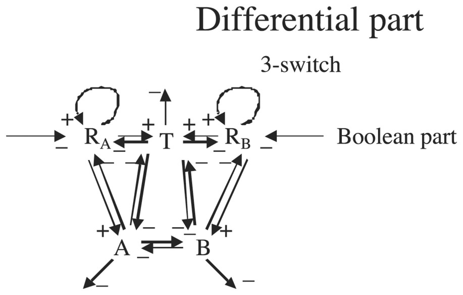
Interaction graph of the epigenetic part as a continuous differential system.
Graph G of Fig. 9 is such that , , , ; G is connected and contains two regulons.
Then we can write the differential system governing the continuous variables T,A,B,RA and RB as follows:
The two first equations correspond to the dynamics of RA (resp RB) whose concentration derivative at time tdRA(t)/dt (resp dRB(t)/dt) results from an auto-catalytic term σRA(t) (resp σRB(t)) diminished by the term (−kT(t)−4kA(t)/5−kB(t)/5) RA(t) (resp (−kT(t)−4kB(t)/5−kA(t)/5) RB(t)) expressing the inhibition by T, A and B, plus a production of growth metabolites term denoted by F(RA(t)) (T(t)+4A(t)/5+B(t))/5)/(T(t)+A(t)+B(t)) (resp F(RB(t))(T(t)+A(t)/5+4B(t)/5)/(T(t)+A(t)+B(t))), by supposing that the RA (resp RB) consumption is competitively inhibited by the bud growth on its side A (resp B) and by the bud growth on the other side and by considering that Kms and s are equal to 1, plus the instantaneous perturbation wPA(t) from its side A (resp B) and wPB(t)/2 from the other side B (resp A), the value of PA(t) (resp PB(t)) being 1 if the pricking treatment occurs on A (resp B) at time t=tP, and 0 elsewhere.
The equations for the apex and cotyledonary buds growth metabolites concentrations just express that their production comes from RA and RB, with a competitive inhibition by the other sources of growth, plus a linear degradation term.
We suppose now for interpreting a minima the experimental results given in Tables 1 and 2 of [33] that F is an allosteric function of order 4 having two successive inflection points (involving that the protein catalysing the production of apex and buds growth metabolites has four catalytic subunits) as allowed by the Monod–Wyman–Changeux equation (see [35] and Fig. 11).
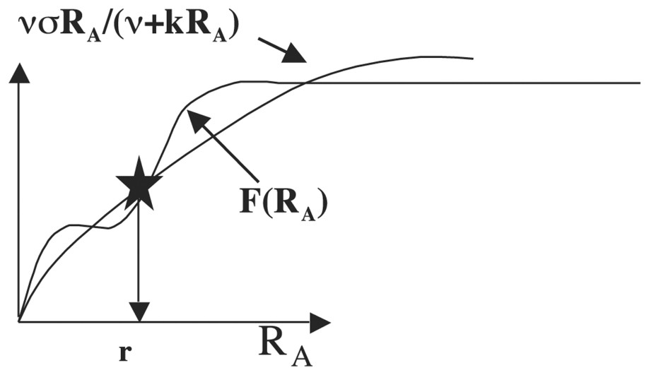
Allosteric function F, which presents two successive inflection points.
If the value of F′ verifies F(r)−rF′(0)<0 and ν<F(r)/r−F′(r)<2 (krF′(r))1/2−ν, then the differential system above possesses at most 16 stationary states, whose 0 is a stable focus, two (respectively (r,0,σr/(ν+kr)) and (0,r,σr/(ν+kr)) are unstable focuses surrounded by limit cycles α and β, and C(r,r,2σr/(ν+kr)) is an attractor (either stable focus, or limit cycle) as shown in Fig. 12, by supposing known the dynamics of the inhibitory three-switch [36] between T, A and B.
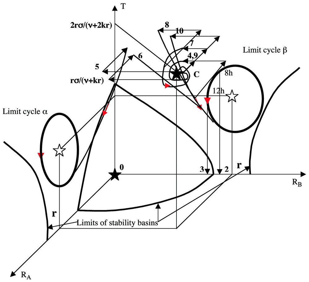
Experimental perturbations in the state space (RA,RB,T).
More generally, if we have an inhibitory n-switch between the Ai's verifying:
The possible configurations of experimental perturbations as reported in Table 1 below and in Tables 1 and 2 of [33] give different trajectories after perturbations, as explained in the following. If nA (resp nB) represents the number of seedlings beginning to elongate on the side of bud A (resp B), then g=(nA−nB)/n, where n=nA+nB, is an asymmetry growth index.
Experimental results about domination growth after decapitation
| Pricking treatment | g | Domination |
| (1) Non-pricked control | 0.02 | A = B |
| (2) 4A with decapitation at onset daylight (dod) | 0.35±0.02 | A<B |
| (3) 4A with decapitation at midday (dm) | 0.08±0.15 | A=B |
| (4) 1A (dod) | 0.01 | A=B |
| (5) 4B (dod) | −0.35 | A>B |
| (6) 1A (1 h) 4B (dod) | 0.39 | A<B |
| (7) 2A (dod) | 0.06 | A=B |
| (8) 2A (1 h) 2A/2B (dod) | 0.32 | A<B |
| (9) 2A (1 h) 2A/2B (3 h) 2A/2B (dod) | 0.05 | A=B |
| (10) 2A (1 h) 2A/2B (3 h) 2A/2B (5 h) 2A/2B (dod) | 0.34 | A<B |
We can make in Fig. 12 above the following observations.
- (1) If the initial conditions are inside the basin of stability of the attractor C, near C, then the whole trajectory without perturbation lies in this basin and tends to the attractor C (where RA≈RB) as time t is tending to infinity. After decapitation without primitive pricking (non-pricked control), A and B buds have the same chance to begin to grow up, then to inhibit the bud growth on the opposite side, hence g≈0.
- (2–3) If we do four pricking treatments on A, then from initial conditions near C we observe a shift to the basin of the limit cycle β and following the decapitation time, we get a B domination if decapitation is done at the onset daylight (dod) and a symmetry in buds growth if it occurs at midday (dm) (see Fig. 12): it is due to the fact that RA and RB after decapitation lies in the basin of the limit cycle β where RB>RA in the first case and are in the basin of the stable focus 0 in the second case.
- (4) If the system is starting near C and if one pricking 1A is done on cotyledon A (resp B), then we suppose that the perturbation results in a decrease of intensity w of RA (resp RB) and in a decrease of intensity w/2 of RB (resp RA) at time tP of pricking; then the variables RA and RB remain in the basin of C.
- (5) If we are doing four pricking treatments on side B, then the point representing the system leaves the basin of C with a decrease of 4w in RA and 2w in RB to go to the basin of the limit cycle β.
- (6) If we do one pricking on side A and 1 h after four prickings on side B, then the system goes in the basin of the limit cycle α and for opposite reasons than for (5) above, RB<RA and A dominates B after decapitation.
- (7) If we do two prickings on side A, then the system remains in the basin of C.
- (8) If we do two prickings on side A and 1 h after two prickings on each side, then the system goes in the basin of the limit cycle β.
- (9) If we do two prickings on side A, 1 h after two prickings on each side and 3 h after two prickings on each side, then the system returns in the basin of C due to the special shape of the trajectory (8) going to the limit cycle β passing near the frontiers of the basin of C.
- (10) If we do two prickings on side A, 1 h after two prickings on each side, 3 h after two prickings on each side and 5 h after anew two prickings on each side, the system goes in the basin of C like in (9) after 4 h, then 5 h after it goes from C to the basin of the limit cycle β.
4 Conclusion
An important first conclusion we have to make explicit in this paper concerns the relationship between the number F of fixed points and the number S of interaction circuits of the interaction matrix W: the problem is in fact to find the best upper bound for F for a given interaction matrix W. This question is related to the famous 16th Hilbert's problem, whose one of the aim is to give an efficient upper bound for the number of limit cycles of a polynomial differential system. Let us summarize the role of the architecture of positive and negative circuits of W on the occurrence of multiple stationary behaviours, as obtained above: if the number of nodes and the number of arcs are the same, there is only one isolated interaction circuit (S=1) in W and either this circuit is negative and the lowest bound (0) for F is reached, or this circuit is positive and the upper bound (21) for F is reached. If the number of nodes is n and the number of arcs is n+1, there is two interaction circuits (S=2) with the following structure: if both circuits are negative, F=0; if there is a positive circuit and a negative circuit disjoint, F=0; if there is a positive circuit intersecting a negative circuit, F=1; if there is a positive circuit intersecting a positive circuit, F=1; if there is two disjoint positive circuits, F=22. If, more generally, the number S of interaction circuits of W is m, then: if all circuits are negative, F=0; if all circuits are positive, 2⩽F⩽2m and if all circuits are positive and disjoint, F=2m. An interesting open problem is now to make exhaustive the determination of F and S and in particular to find the circumstances (related to the circuits structure) in which we can relate the number of intersecting and isolated circuits to F. A conjecture we could make is that F=2c, where c is the number of not-singleton connected components of the interaction graph G having at least one positive loop: it holds for the lactose, Arabidopsis, phage μ and gastrulation regulatory systems. The approach for solving this open problem could consist in finding coherent relationships between analogous properties discovered independently for continuous and Boolean versions of regulatory networks [4–9].
The second conclusion concerns the practical use of the presented results; a geneticist can for example exploit the minimality results in the following sense: we have shown in the paper that it would be possible to characterize the minimal interaction matrices having certain state vectors as fixed points. The determination of these matrices is not unique, but permits to focus on a certain important equivalence class to which the expected matrix has to belong. This considerably restricts the choice of the possible interaction matrices compatible with observed fixed points, when it is impossible to directly get from experiments all interaction coefficients, but when it is only possible to observe the phenomenology of fixed points or limit cycles. This corresponds in genetics to the observation of stationary expression behaviours (for example from bio-array imaging) without experimental measure of the inhibitory and activatory coefficients of repressors and promoters. The possibility to obtain (even in an equivalence class) a sketch of the interaction matrix permits to construct (by randomising in a Bayesian way the unknown coefficients of ) more complicated interaction matrices, then to test if they still have the observed states as fixed points and finally keep or reject definitively the so-tested matrices and propose further experimental strategies refining the knowledge about the interaction structure of a genetic regulatory network and then answer crucial biological questions like the relationship between genetic expression and recombination [16,38–40] (the crossing-over and translocations break points seeming correlated with the ubiquitory genes expression sites) or the relative parts taken by genetic and epigenetic forces in morphogenesis (embryogenesis or tumorogenesis). The last (but not the least) application of the interaction matrices introduced above is the ability to calculate the barycentre between two matrices by using classical (spectral or L2) distances between matrices, then we could build phylogenic trees among a set of species avoiding the complex problems coming from the non-unicity of L1 (Hamming or Manhattan) barycentres met in the sequence based phylogenic trees. The interaction based phylogenic trees could reflect more the genomic function than the genomic anatomy hence could explain more deeply the evolution trends.
Acknowledgements
We have done this work thanks to the support of the National Network for Technology Research RNTS ‘Technologies for Health’ from the French Ministry of Research.