Stochastic models for circadian rhythms: effect of molecular noise on periodic and chaotic behaviour

Didier Gonze; José Halloy; Jean-Christophe Leloup; Albert Goldbeter

doi:10.1016/S1631-0691(03)00016-7

Biological modelling / Biomodélisation

Stochastic models for circadian rhythms: effect of molecular noise on periodic and chaotic behaviour
[Modèles stochastiques pour les rythmes circadiens : effet du bruit moléculaire sur les comportements périodiques et chaotiques]

Didier Gonze ¹ ; José Halloy ¹ ; Jean-Christophe Leloup ¹ ; Albert Goldbeter ¹

¹ Unité de chronobiologie théorique, faculté des sciences, université libre de Bruxelles, Campus Plaine, CP 231, B1050 Brussels, Belgium

Comptes Rendus. Biologies, Volume 326 (2003) no. 2, pp. 189-203.

Résumés

Anglais
Français

Circadian rhythms are endogenous oscillations that occur with a period close to 24 h in nearly all living organisms. These rhythms originate from the negative autoregulation of gene expression. Deterministic models based on such genetic regulatory processes account for the occurrence of circadian rhythms in constant environmental conditions (e.g., constant darkness), for entrainment of these rhythms by light-dark cycles, and for their phase-shifting by light pulses. When the numbers of protein and mRNA molecules involved in the oscillations are small, as may occur in cellular conditions, it becomes necessary to resort to stochastic simulations to assess the influence of molecular noise on circadian oscillations. We address the effect of molecular noise by considering the stochastic version of a deterministic model previously proposed for circadian oscillations of the PER and TIM proteins and their mRNAs in Drosophila. The model is based on repression of the per and tim genes by a complex between the PER and TIM proteins. Numerical simulations of the stochastic version of the model are performed by means of the Gillespie method. The predictions of the stochastic approach compare well with those of the deterministic model with respect both to sustained oscillations of the limit cycle type and to the influence of the proximity from a bifurcation point beyond which the system evolves to a stable steady state. Stochastic simulations indicate that robust circadian oscillations can emerge at the cellular level even when the maximum numbers of mRNA and protein molecules involved in the oscillations are of the order of only a few tens or hundreds. The stochastic model also reproduces the evolution to a strange attractor in conditions where the deterministic PER–TIM model admits chaotic behaviour. The difference between periodic oscillations of the limit cycle type and aperiodic oscillations (i.e. chaos) persists in the presence of molecular noise, as shown by means of Poincaré sections. The progressive obliteration of periodicity observed as the number of molecules decreases can thus be distinguished from the aperiodicity originating from chaotic dynamics. As long as the numbers of molecules involved in the oscillations remain sufficiently large (of the order of a few tens or hundreds, or more), stochastic models therefore provide good agreement with the predictions of the deterministic model for circadian rhythms.

Les rythmes circadiens sont des oscillations endogènes qui se produisent avec une période proche de 24 h chez la plupart des organismes vivants. Ces rythmes résultent de l'autorégulation négative de l'expression de gènes de l'horloge circadienne. Des modèles déterministes fondés sur de tels processus de régulation génétique rendent compte de l'existence de rythmes circadiens dans des conditions d'environnement constant (par exemple, l'obscurité continue), de l'entraı̂nement de ces rythmes par des cycles lumière–obscurité, et de leur déphasage par des impulsions de lumière. Lorsque le nombre de molécules d'ARN messagers et de protéines impliquées dans le mécanisme des oscillations est faible, comme cela peut se produire dans les conditions cellulaires, il devient nécessaire de recourir à des simulations stochastiques pour déterminer l'influence du bruit moléculaire sur les rythmes circadiens. Nous étudions l'effet du bruit moléculaire en considérant la version stochastique d'un modèle déterministe précédemment proposé pour les oscillations circadiennes des protéines PER et TIM et de leurs ARN messagers chez la drosophile. Ce modèle est fondé sur la répression des gènes per et tim par un complexe entre les protéines PER et TIM. Les simulations numériques de la version stochastique de ce modèle sont effectuées au moyen de la méthode de Gillespie. Les prédictions de l'approche stochastique sont en accord avec celles fournies par l'approche déterministe, tant pour ce qui concerne les oscillations entretenues de type cycle limite que pour l'influence de la proximité d'un point de bifurcation au-delà duquel le système évolue vers un état stationnaire stable. Les simulations stochastiques indiquent que des rythmes circadiens robustes peuvent émerger au niveau cellulaire déjà lorsque le nombre maximum de molécules d'ARN messagers et de protéines impliquées dans les oscillations est de l'ordre de quelques dizaines ou centaines seulement. Le modèle stochastique reproduit également l'évolution vers un attracteur étrange dans les conditions où le modèle déterministe PER–TIM admet un comportement chaotique. La différence entre les oscillations périodiques de type cycle limite et les oscillations apériodiques – c'est-à-dire le chaos – persiste en présence de bruit moléculaire, comme l'indiquent les sections de Poincaré obtenues pour les deux types de comportement dynamique. La disparition progressive de la périodicité, qu'on observe à mesure que le nombre de molécules diminue, peut donc être distinguée de l'apériodicité résultant de la dynamique chaotique. Aussi longtemps que le nombre de molécules impliquées dans les oscillations demeure suffisamment grand (de l'ordre de quelques dizaines, centaines, ou plus), les modèles stochastiques fournissent ainsi un bon accord avec les prédictions des modèles déterministes pour les rythmes circadiens.

Métadonnées

Reçu le : 2002-10-09
Accepté le : 2002-12-17
Publié le : 2003-02-01

PMID

DOI : 10.1016/S1631-0691(03)00016-7

Keywords: circadian rhythms, stochastic simulations, molecular noise, robustness, chaos
Mot clés : rythmes circadiens, simulations stochastiques, bruit moléculaire, robustesse, chaos

Affiliations des auteurs :

Didier Gonze ¹ ; José Halloy ¹ ; Jean-Christophe Leloup ¹ ; Albert Goldbeter ¹

¹ Unité de chronobiologie théorique, faculté des sciences, université libre de Bruxelles, Campus Plaine, CP 231, B1050 Brussels, Belgium

@article{CRBIOL_2003__326_2_189_0,
     author = {Didier Gonze and Jos\'e Halloy and Jean-Christophe Leloup and Albert Goldbeter},
     title = {Stochastic models for circadian rhythms: effect of molecular noise on periodic and chaotic behaviour},
     journal = {Comptes Rendus. Biologies},
     pages = {189--203},
     publisher = {Elsevier},
     volume = {326},
     number = {2},
     year = {2003},
     doi = {10.1016/S1631-0691(03)00016-7},
     language = {en},
}

TY  - JOUR
AU  - Didier Gonze
AU  - José Halloy
AU  - Jean-Christophe Leloup
AU  - Albert Goldbeter
TI  - Stochastic models for circadian rhythms: effect of molecular noise on periodic and chaotic behaviour
JO  - Comptes Rendus. Biologies
PY  - 2003
SP  - 189
EP  - 203
VL  - 326
IS  - 2
PB  - Elsevier
DO  - 10.1016/S1631-0691(03)00016-7
LA  - en
ID  - CRBIOL_2003__326_2_189_0
ER  -

%0 Journal Article
%A Didier Gonze
%A José Halloy
%A Jean-Christophe Leloup
%A Albert Goldbeter
%T Stochastic models for circadian rhythms: effect of molecular noise on periodic and chaotic behaviour
%J Comptes Rendus. Biologies
%D 2003
%P 189-203
%V 326
%N 2
%I Elsevier
%R 10.1016/S1631-0691(03)00016-7
%G en
%F CRBIOL_2003__326_2_189_0

Didier Gonze; José Halloy; Jean-Christophe Leloup; Albert Goldbeter. Stochastic models for circadian rhythms: effect of molecular noise on periodic and chaotic behaviour. Comptes Rendus. Biologies, Volume 326 (2003) no. 2, pp. 189-203. doi : 10.1016/S1631-0691(03)00016-7. https://comptes-rendus.academie-sciences.fr/biologies/articles/10.1016/S1631-0691(03)00016-7/

Version originale du texte intégral

1 Introduction

Most living organisms, from cyanobacteria to insects, plants and mammals, have developed the capability of generating autonomously sustained oscillations with a period close to 24 h. These oscillations, known as circadian rhythms, are endogenous because they can occur in constant environmental conditions, e.g., constant darkness [1,2]. Experimental studies during the last decade have shed much light on the molecular mechanism of circadian rhythms [3]. Initial studies pertained to the fly Drosophila [4,5] and the fungus Neurospora [3]. Molecular studies of circadian rhythms have since been extended to cyanobacteria, plants and mammals [6,7]. In all cases investigated so far, the molecular mechanism of circadian oscillations relies on the negative autoregulation exerted by a protein on the expression of its gene [3–8]. Thus, in Drosophila, the proteins PER and TIM form a complex that indirectly represses the activation of the per and tim genes, while in Neurospora it is the FRQ protein that represses the expression of its gene frq [3,6]. The situation in mammals resembles that observed in Drosophila, but instead of TIM it is the CRY protein that forms a regulatory complex with a PER protein to inhibit the expression of the per genes [7]. Light can entrain circadian rhythms by inducing degradation of the TIM protein in Drosophila, and expression of the frq and per genes in Neurospora and mammals, respectively [3–7].

A number of mathematical models for circadian rhythms have been proposed [9–15] on the basis of these experimental observations. These models are of a deterministic nature and take the form of a system of coupled ordinary differential equations. The models predict that in a certain range of parameter values the genetic control network undergoes sustained oscillations of the limit cycle type corresponding to the circadian rhythm, whereas outside this range the gene network operates in a stable steady state. The question arises as to whether deterministic models are always appropriate for the description of circadian clocks [16]. Indeed, the number of molecules involved in the regulatory mechanism producing circadian rhythms at the cellular level may well be reduced. This number could vary from a few thousands down to hundreds and even a few tens of protein or messenger RNA molecules in each rhythm-producing cell. At such low concentrations it is more appropriate to resort to a stochastic approach to study the molecular bases of the oscillatory phenomenon.

In a previous publication [17], we compared the stochastic and deterministic versions of a core molecular model for circadian oscillations based on the negative regulation exerted by a protein on the expression of its gene. Stochastic simulations were performed by means of the Gillespie algorithm [18,19] after decomposing the deterministic model into elementary steps. We studied the effect of molecular noise by assessing the robustness of circadian oscillations as a function of the number of interacting molecules. We showed that robust circadian rhythmicity could already occur when the maximum numbers of mRNA and clock protein molecules are in the tens and hundreds, respectively. Cooperativity of repression and periodic forcing by light-dark cycles enhance the robustness of circadian oscillations. In subsequent work [20], we compared two stochastic versions of this core model, one fully developed into elementary steps, and the other non-developed. We showed that stochastic treatment of these two versions of the model for circadian rhythms yields similar results.

The purpose of the present paper is to extend our comparison of deterministic and stochastic models for circadian oscillations, by considering a more detailed model for the Drosophila circadian clock incorporating the formation of a complex between the PER and TIM proteins. Although this model does not take into account other proteins such as CLOCK and CYC involved in the circadian oscillatory mechanism, it is nevertheless more realistic than the core model and accounts for a larger number of experimental observations. Moreover, this extended model predicts the possibility of autonomous chaotic behaviour [21]. Such a property will allow us to assess the effect of molecular noise not only on periodic but also on chaotic oscillations.

We first present in Section 2 the deterministic and stochastic versions of the molecular model for circadian rhythms. In the stochastic version we introduce molecular noise without decomposing the deterministic mechanism into detailed reaction steps. The results of stochastic simulations performed by means of the Gillespie method [18,19] are presented in Section 3 for the case of periodic behaviour. We assess the role of fluctuations by determining the effect of the number of mRNA and protein molecules on circadian rhythmicity. In Section 4 we examine how the proximity from a bifurcation point influences the robustness of the oscillations with respect to molecular noise. How such a noise affects chaotic behaviour is examined in Section 5. Section 6 is devoted to a comparative discussion of deterministic versus stochastic simulations.

2 Deterministic and stochastic versions of the molecular model for circadian oscillations

2.1 Deterministic model for circadian oscillations

We consider a ten-variable model previously proposed for circadian oscillations of the PER and TIM proteins and of per and tim mRNAs in Drosophila [9,10]. The model, schematised in Fig. 1, is based on the negative feedback exerted by the complex between the nuclear PER and TIM proteins on the expression of their genes. For each of these proteins the gene is first transcribed in the nucleus into messenger RNA (mRNA). The latter is transported into the cytosol where it is degraded and translated into the protein P₀ (T₀). The protein PER (TIM) undergoes multiple phosphorylation, from P₀ into P₁ (T₀ into T₁) and from P₁ into P₂ (T₁ into T₂). These modifications, catalysed by a protein kinase, are reverted by a phosphatase. The fully phosphorylated form of the proteins is marked up for degradation and forms a complex (C), which is transported into the nucleus in a reversible manner. The nuclear form of the PER–TIM complex (C_N) represses the transcription of the per and tim genes. Recent experiments indicate that repression is in fact of indirect nature: the CLOCK and CYC proteins promote the expression of the per and tim genes and are prevented from exerting this activation when forming a complex with PER and TIM [3–7]. In the model, the variables are the concentrations of the mRNAs (M_P and M_T), of the various forms of the PER and TIM proteins (P₀, P₁, P₂, T₀, T₁, T₂), and of the cytosolic (C) and nuclear (C_N) forms of the PER–TIM complex. The temporal evolution of these concentration variables is governed by a system of 10 kinetic equations that are listed in Appendix A (see [9,10] for further details).

Fig. 1
Model for circadian rhythms in Drosophila. The model is based on the negative regulation of the per and tim genes by a complex between the PER and TIM proteins [11]. The per (M_P) and tim (M_T) mRNAs are synthesised in the nucleus and transferred into the cytosol, where they accumulate at the maximum rates v_sP and v_sT, respectively; there they are degraded enzymatically at the maximum rates v_mP and v_mT, with the Michaelis constants K_mP and K_mT. The rates of synthesis of the PER and TIM proteins, respectively proportional to M_P and M_T, are characterised by the apparent first-order rate constants k_sP and k_sT. Parameters V_iP, V_iT and K_iP, K_iT (i=1,…,4) denote the maximum rate and Michaelis constant of the kinase(s) and phosphatase(s) involved in the reversible phosphorylation of P₀ (T₀) into P₁ (T₁) and P₁ (T₁) into P₂ (T₂), respectively. The fully phosphorylated forms (P₂ and T₂) are degraded by enzymes of maximum rate v_dP, v_dT and Michaelis constants K_dP, K_dT, and reversibly form a complex C (with the forward and reverse rate constants k₃, k₄), which is transported into the nucleus at a rate characterised by the apparent first-order rate constant k₁. Transport of the nuclear form of the PER–TIM complex (C_N) into the cytosol is characterised by the apparent first-order rate constant k₂. The negative feedback exerted by the nuclear PER–TIM complex on per and tim transcription is described by an equation of the Hill type, in which n denotes the degree of cooperativity, and K_IP and K_IT the threshold constants for repression.

The deterministic PER–TIM model accounts for the occurrence of sustained oscillations in continuous darkness. When taking into account the control exerted by light on the maximum protein degradation rate v_dT, the model also accounts for entrainment of circadian oscillations by light-dark cycles and for their phase shifting by pulses of light. Circadian oscillations have also been obtained in more detailed models based on indirect repression and involving additional clock gene products such as CLOCK and CYC ([14,15], J.-C. Leloup and A. Goldbeter, submitted for publication).

As indicated above, besides periodic oscillations, the model of Fig. 1 is also capable of generating autonomous chaos in conditions corresponding to continuous darkness. Although this behaviour is probably not of physiological significance [21], it provides us with the rare opportunity of testing the effect of molecular noise on chaotic behaviour in a realistic model based on genetic regulation.

2.2 Stochastic version of the model for circadian oscillations

To assess the effect of molecular noise, we describe the reaction steps as stochastic birth and death processes [22]. Numerical simulations of the temporal evolution of the genetic control system are performed by means of the Gillespie method [17,18]. Besides other approaches [23–25], this method has been used to determine the dynamics of chemical [24,25] biochemical [26] or genetic systems [27] in the presence of molecular noise. The Gillespie method associates a probability with each reaction step; at each time step the algorithm randomly determines the reaction that takes place according to its probability, as well as the time interval to the next reaction step. The numbers of molecules of the different reacting species as well as the probabilities are updated at each time step. In this approach [18,19], a parameter denoted $Ω$ controls the number of molecules present in the system. Using the Gillespie method we performed stochastic simulations of the model described in section 2.1.

Our previous analysis of a core molecular model for circadian rhythms showed [17] that similar results are obtained when decomposing the deterministic model into elementary steps (developed model) or when the deterministic model is not decomposed into such steps and non-linear kinetic functions are simply included in the probabilities associated with the global reaction steps (non-developed model). Because it is much easier to handle, we shall therefore restrict our stochastic analysis to such a non-developed version of the model schematised in Fig. 1.

The non-linear terms appearing in the kinetic equations (A.1) listed in Appendix A represent compact kinetic expressions obtained after application of quasi-steady-state hypotheses on enzyme–substrate or gene–repressor complexes. The resulting expressions are of the Michaelis–Menten type for enzyme reaction rates, or of the Hill type for cooperative binding of the repressor (here, the nuclear PER–TIM complex) to the gene promoter. We attribute to each linear or non-linear term of the kinetic equations a probability of occurrence of the corresponding reaction. These reactions and their associated probability are listed in Table 1 in Appendix A. Thus reaction (1) corresponds to the transcription of the per gene into per mRNA, M_P; the occurrence of this reaction with a probability w₁ results in increasing by 1 the number of molecules of M_P. Reaction (4) results in increasing by one the number of P₁ molecules and decreasing by one the number of molecules of P₀.

Reaction number	Reaction step	Probability of reaction
1	$\begin{matrix} v_{sP} \\ \to \end{matrix} M_{P}$	$w_{1} = (v_{sP} \times Ω) \frac{{(K_{IP} \times Ω)}^{n}}{{(K_{IP} \times Ω)}^{n} + C_{N}^{n}}$
2	$M_{P} \begin{matrix} v_{mP} \\ \to \end{matrix}$	$w_{2} = (v_{mP} \times Ω) \frac{M_{P}}{(K_{mP} \times Ω) + M_{P}}$
3	$M_{P} \begin{matrix} k_{sP} \\ \to \end{matrix} P_{0}$	w₃=k_sP×M_P
4	$P_{0} \begin{matrix} V_{1 P} \\ \to \end{matrix} P_{1}$	$w_{4} = (V_{1 P} \times Ω) \frac{P_{0}}{(K_{1 P} \times Ω) + P_{0}}$
5	$P_{1} \begin{matrix} V_{2 P} \\ \to \end{matrix} P_{0}$	$w_{5} = (V_{2 P} \times Ω) \frac{P_{1}}{(K_{2 P} \times Ω) + P_{1}}$
6	$P_{1} \begin{matrix} V_{3 P} \\ \to \end{matrix} P_{2}$	$w_{6} = (V_{3 P} \times Ω) \frac{P_{1}}{(K_{3 P} \times Ω) + P_{1}}$
7	$P_{2} \begin{matrix} V_{4 P} \\ \to \end{matrix} P_{1}$	$w_{7} = (V_{4 P} \times Ω) \frac{P_{2}}{(K_{4 P} \times Ω) + P_{2}}$
8	$P_{2} + T_{2} \begin{matrix} k_{3} \\ \to \end{matrix} C$	$w_{8} = k_{3} \times P_{2} \times T_{2} / Ω$
9	$C \begin{matrix} k_{4} \\ \to \end{matrix} P_{2} + T_{2}$	w₉=k₄×C
10	$P_{2} \begin{matrix} V_{dP} \\ \to \end{matrix}$	$w_{10} = (V_{dP} \times Ω) \frac{P_{2}}{(K_{dP} \times Ω) + P_{2}}$
11	$\begin{matrix} V_{sT} \\ \to \end{matrix} M_{T}$	$w_{11} = (v_{sT} \times Ω) \frac{{(K_{IT} \times Ω)}^{n}}{{(K_{IT} \times Ω)}^{n} + C_{N}^{n}}$
12	$M_{T} \begin{matrix} V_{mT} \\ \to \end{matrix}$	$w_{12} = (V_{mT} \times Ω) \frac{M_{T}}{(K_{mT} \times Ω) + M_{T}}$
13	$M_{T} \begin{matrix} V_{sT} \\ \to \end{matrix} T_{0}$	w₁₃=k_sT×M_T
14	$T_{0} \begin{matrix} V_{1 T} \\ \to \end{matrix} T_{1}$	$w_{14} = (V_{1 T} \times Ω) \frac{T_{0}}{(K_{1 T} \times Ω) + T_{0}}$
15	$T_{1} \begin{matrix} V_{2 T} \\ \to \end{matrix} T_{0}$	$w_{15} = (V_{2 T} \times Ω) \frac{T_{1}}{(K_{2 T} \times Ω) + T_{1}}$
16	$T_{1} \begin{matrix} V_{3 T} \\ \to \end{matrix} T_{2}$	$w_{16} = (V_{3 T} \times Ω) \frac{T_{1}}{(K_{3 T} \times Ω) + T_{1}}$
17	$T_{2} \begin{matrix} V_{4 T} \\ \to \end{matrix} T_{1}$	$w_{17} = (V_{4 T} \times Ω) \frac{T_{2}}{(K_{4 T} \times Ω) + T_{2}}$
18	$T_{2} \begin{matrix} V_{dT} \\ \to \end{matrix}$	$w_{18} = (V_{dT} \times Ω) \frac{T_{2}}{(K_{dT} \times Ω) + T_{2}}$
19	$C \begin{matrix} k_{1} \\ \to \end{matrix} C_{N}$	w₁₉=k₁×C
20	$C_{N} \begin{matrix} k_{2} \\ \to \end{matrix} C$	w₂₀=k₂×C_N
21	$M_{P} \begin{matrix} k_{d} \\ \to \end{matrix}$	w₂₁=k_d×M_P
22	$P_{0} \begin{matrix} k_{d} \\ \to \end{matrix}$	w₂₂=k_d×P₀
23	$P_{1} \begin{matrix} k_{d} \\ \to \end{matrix}$	w₂₃=k_d×P₁
24	$P_{2} \begin{matrix} k_{d} \\ \to \end{matrix}$	w₂₄=k_d×P₂
25	$M_{T} \begin{matrix} k_{d} \\ \to \end{matrix}$	w₂₅=k_d×M_T
26	$T_{0} \begin{matrix} k_{d} \\ \to \end{matrix}$	w₂₆=k_d×T₀
27	$T_{1} \begin{matrix} k_{d} \\ \to \end{matrix}$	w₂₇=k_d×T₁
28	$T_{2} \begin{matrix} k_{d} \\ \to \end{matrix}$	w₂₈=k_d×T₂
29	$C \begin{matrix} k_{dC} \\ \to \end{matrix}$	w₂₉=k_dC×C
30	$C_{N} \begin{matrix} k_{dN} \\ \to \end{matrix}$	w₃₀=k_dN×C_N

In contrast to the treatment presented in our previous work [17], here we do not decompose the binding of the repressor to the gene promoter into successive elementary steps, and rather retain the Hill function description for cooperative repression by the nuclear PER–TIM complex C_N (steps (1) and (11)). A similar global approach is taken for describing degradation of per and tim mRNAs (reactions (2) and (12)), translation of mRNAs into proteins P₀ and T₀ (reactions (3) and (13)), phosphorylation of P₀ and T₀ into P₁ and T₁ (reactions (4) and (14)) and of P₁ and T₁ into P₂ and T₂ (reactions (6) and (16)), as well as dephosphorylation of P₁ and T₁ into P₀ and T₀ (reactions 5 and 15) and of P₂ and T₂ into P₁ and T₁ (reactions (7) and (17)), enzymatic degradation of P₂ and T₂ (reactions (10) and (18)), reversible formation of the complex C (reactions 8 and 9), and reversible transport of complex C into and out of the nucleus (reactions (19) and (20)). Steps (21)–(30) relate to non-specific degradation of the various mRNA or protein species. Reactions (2), (4)–(7), (10), (12), and (14)–(18) are of the Michaelian type; reaction (8) is of bimolecular nature, while reactions (3), (9), (13) and (19)–(30) correspond to linear kinetics.

3 Effect of molecular noise on periodic oscillations

Before dealing with the effect of molecular noise, let us recall the predictions of the deterministic model governed by equations (A.1). Typical circadian oscillations predicted by this model are shown in Fig. 2A (middle panel). These oscillations correspond to the evolution toward a limit cycle (Fig. 2A, left panel) shown here as a projection onto the plane formed by the concentrations of per mRNA (M_P) and nuclear PER–TIM complex (C_N). Because the behaviour is periodic and deterministic (i.e. oscillations occur in the absence of molecular noise), the histogram of periods yields a single line corresponding to a circadian period close to 24 h (Fig. 2A, right panel).

Fig. 2
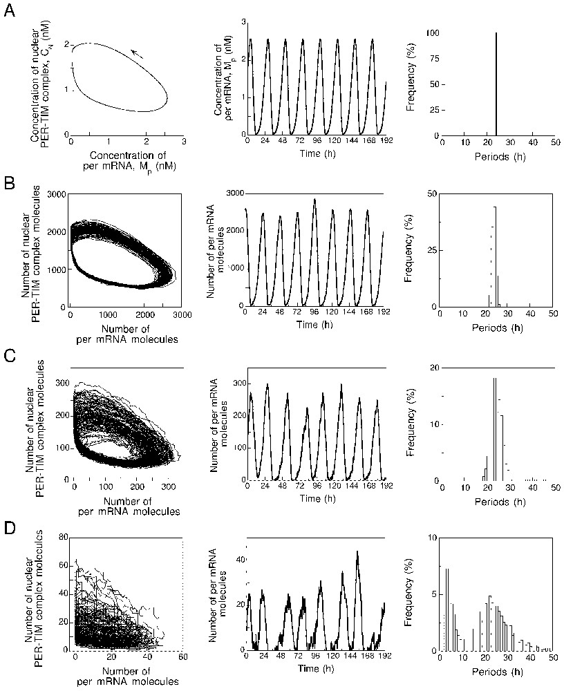
Sustained oscillations predicted by the deterministic and stochastic versions of the model for circadian rhythms. (A) Limit cycle obtained in the 10-variable deterministic model governed by equations (A.1), shown as a projection onto the M_P–C_N phase plane (left panel); the arrow indicates the direction of movement along the closed trajectory. Equations (A.1) and parameter values are listed in Appendix A. Middle panel: sustained oscillations of per mRNA (M_P) corresponding to the limit cycle in the left panel. Right panel: histogram of periods. Here, in the absence of molecular noise, the deterministic model yields a single line corresponding to the periodic circadian oscillations. (B)–(D) Limit cycle (left panel), sustained oscillations (represented by the time course of the number of per mRNA molecules), and histograms of periods predicted by the stochastic model for values of parameter $Ω$ decreasing from 1000 (B) to 100 (C) and 10 (D). The results, obtained in the presence of molecular noise, should be compared with those obtained with the deterministic model in (A). Numerical simulations in panels (B)–(D) were performed by means of the Gillespie method [16,17] with the stochastic model listed in Table 1 in Appendix A. As in the following figures stochastic simulations were performed for 2500 h, which corresponds to some 100 successive cycles. For period histograms, the period was determined as the time interval separating two successive upward crossings of the mean level of mRNA or clock protein.

Turning to the effect of molecular noise, we now consider the dynamic behaviour of the stochastic version of the PER–TIM model for circadian rhythms. Shown in panels B–D in Fig. 2 are the limit cycles (left panels), sustained oscillations of per mRNA (middle panels), and histograms of periods (right panels) obtained by stochastic simulations for $Ω = 1000$ (B), 100 (C) and 10 (D). For these values of $Ω$ , the numbers of molecules of nuclear PER–TIM complex and per mRNA vary in the range 500–2500 and 0–3000, 50–300 and 0–300, and 0–60 and 0–50, respectively.

The data presented in Fig. 2 show that the circadian oscillatory behaviour predicted by the deterministic model is recovered when using the stochastic model for circadian rhythms. The mere effect of molecular noise is to increase the effective thickness of the limit cycle. The results further indicate that robust circadian oscillations are still produced by the stochastic model when the maximum numbers of mRNA and protein molecules are in the order of hundreds. It is only when these numbers decrease down to a few tens that noise begins to overcome rhythmicity, even though oscillations still subsist (Fig. 2D); the period histogram is then much wider but still presents a maximum close to a circadian value.

Another way to illustrate the effect of molecular noise is to draw a histogram of frequencies of passage through the different points in the phase plane. In the deterministic case, such a plot would yield the same frequency of passage through all points of the limit cycle, because these are all visited the same number of times. In the presence of noise, some regions of the phase space are visited more often than others where dispersion is strong. This results in the occurrence of peaks in the frequency of passage, as shown in Fig. 3A. The bottom part of Fig. 3A shows a contour plot in the plane (per mRNA molecules versus nuclear PER–TIM complexes). The contour plot is obtained by projecting onto this plane the intersections of the histogram with 50 parallel planes, corresponding to equidistant frequencies. For the sake of clarity the contour plot is rotated by 90° and shown enlarged in Fig. 3B. The most frequently visited regions in the phase plane correspond to the decrease in nuclear PER–TIM levels and rise in per mRNA. Largest dispersion occurs when mRNA decreases and PER–TIM levels rise.

Fig. 3
Probability of passage of a trajectory in a given region of the phase space in the presence of molecular noise, in conditions corresponding to the evolution to the limit cycle shown in Fig. 2C (left panel). Molecular noise induces a dispersion of the trajectories around the deterministic limit cycle (Fig. 2A, left panel); the probability of passage is highest where the trajectories are less dispersed. The bottom part of Fig. 3A shows contour lines of the probability of passage in different regions of the phase plane (per mRNA molecules, nuclear PER–TIM complex molecules). The contour plot contains 50, equidistant isoprobability lines between minimum and maximum probability. Panel B shows an enlargement of the contour plot, rotated by 90° for the sake of comparison with the limit cycles shown in the left panels of Fig. 2. Parameter values are as in Fig. 2, with $Ω = 100$ .

4 Influence of the vicinity of a bifurcation point

The question arises as to whether the proximity from a bifurcation point may influence the robustness of circadian oscillations with respect to molecular noise. To address this issue, we first construct in Fig. 4 a bifurcation diagram showing the onset of limit cycle oscillations as a function of the maximum rate of TIM degradation, v_dT, for the deterministic model governed by equations (A.1). The state of the system is represented in Fig. 4 by a single variable, the concentration of per mRNA. Below $v_{dT} = 0.46 nM h^{- 1}$ , the system evolves toward a stable steady state. Above this critical bifurcation value, limit cycle oscillations occur. The diagram shows the envelope of the oscillations: the upper and lower branches yield the maximum and minimum values of per mRNA concentration as a function of v_dT in the course of oscillations.

Fig. 4
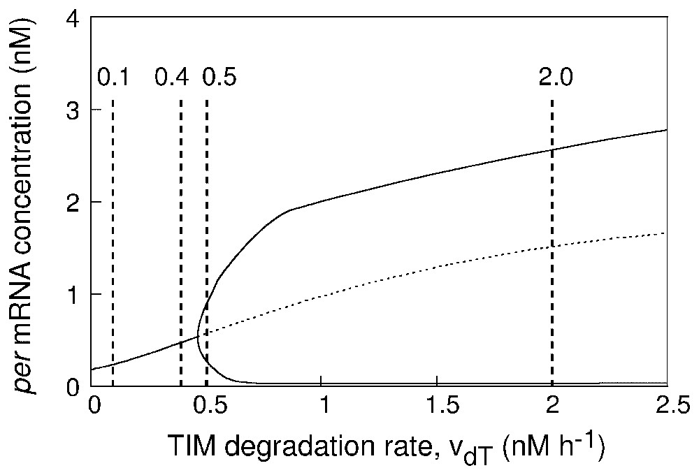
Bifurcation diagram showing the onset of circadian oscillations in the deterministic model as a function of parameter v_dT which measures the maximum rate of TIM degradation. The curve shows the steady-state level of per mRNA, stable (solid line) or unstable (dashed line), as well as the maximum and minimum concentration of per mRNA in the course of sustained circadian oscillations. The vertical dashed lines refer to the four values considered for v_dT in Fig. 5, in panels (A)–(D), respectively. The diagram is established by means of the program AUTO [32] applied to equations (A.1) listed in Appendix A. Parameter values are as in Fig. 2.

The results of stochastic simulations performed with increasing values of parameter v_dT are shown in Fig. 5 in the form of dynamics in the phase plane (right panels) or time series (left panels). The steady state or limit cycle predicted by the deterministic model for the corresponding parameter values is shown in the phase plane by a white dot or a white curve, respectively. The four panels in Fig. 5 correspond to the four v_dT values indicated by dashed vertical lines in Fig. 4. For $v_{dT} = 0.1 nM h^{- 1}$ , the deterministic system evolves to a stable steady state far from the bifurcation point; stochastic simulations show low-amplitude fluctuations around the deterministic steady state (Fig. 5A). For $v_{dT} = 0.4 nM h^{- 1}$ , the deterministic system evolves to a stable steady state close to the bifurcation point; stochastic simulations show fluctuations of larger amplitude around the deterministic steady state (Fig. 5B). For $v_{dT} = 0.5 nM h^{- 1}$ , the deterministic system undergoes limit cycle oscillations of reduced amplitude just beyond the bifurcation point; stochastic simulations show small-amplitude, noisy oscillations around the deterministic limit cycle (Fig. 5C), which resemble the fluctuations shown in Fig. 5B. Finally, for $v_{dT} = 2.0 nM h^{- 1}$ , the deterministic system undergoes limit cycle oscillations of large amplitude far from the bifurcation point; stochastic simulations show large-amplitude, relatively less noisy oscillations around the deterministic limit cycle (Fig. 5D).

Fig. 5
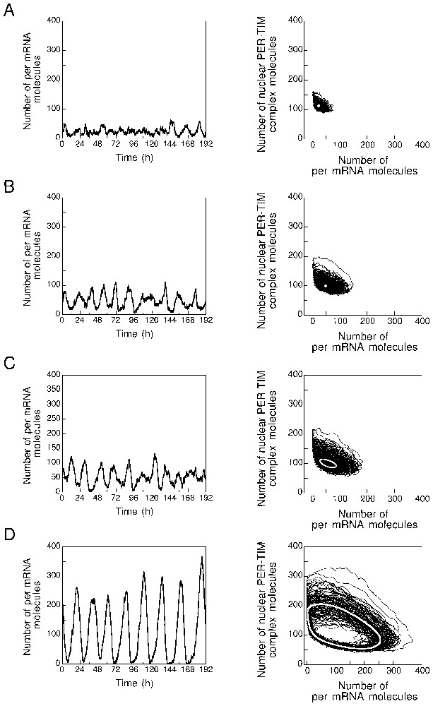
Effect of the proximity from a bifurcation point on the effect of molecular noise in the stochastic model for circadian rhythms. The different panels are established for the four increasing values of parameter v_dT shown in Fig. 4: 0.1 (A), 0.4 (B), 0.5 (C) and 2 (D); these values, to be multiplied by $Ω$ , are expressed here in molecules per hour. The right panels show the evolution in the phase plane while the left panels represent the corresponding temporal evolution of the number of per mRNA molecules. (A) Fluctuations around a stable steady state. (B) Fluctuations around a stable steady state for a value of v_dT close to the bifurcation point which lies around 0.47 molecules per hour. Damped oscillations occur in these conditions when the system is displaced from the stable steady state. In (A) and (B), the white dot represents the stable steady state predicted by the deterministic version of the model in corresponding conditions. (C) Oscillations observed close to the bifurcation point. (D) Oscillations observed further from the bifurcation point, well into the domain of sustained oscillations. In (C) and (D) the thick white curve represents the limit cycle predicted by the deterministic version of the model governed by equations (A.1), in corresponding conditions, for the same values of v_dT expressed in $nM h^{- 1}$ . The smaller amplitude of the limit cycle in (C) as compared to the limit cycle in (D) is associated with an increased influence of molecular noise. The curves are obtained by means of the Gillespie algorithm applied to the model of Table 1 (see Appendix A). Besides v_dT, parameter values are as in Fig. 2.

The data in Fig. 5 indicate that stochastic simulations allow us to recover the dynamics predicted by the deterministic model. Below a critical parameter value, the system displays low-amplitude fluctuations around a stable steady state, while above this value sustained oscillations occur. Moreover, the effect of fluctuations is enhanced by the proximity from the bifurcation point.

5 Effect of molecular noise on chaotic behaviour

We have previously reported the occurrence of autonomous chaos in the deterministic model of Fig. 1 [21]. Thus, for some parameter values, in conditions corresponding to continuous darkness, sustained aperiodic oscillations occur in this model, which correspond to the evolution toward a strange attractor in the phase space (see Fig. 6A). This phenomenon provides us with the rare opportunity to assess the effect of molecular noise on chaotic behaviour in a realistic biochemical model. Shown in panels B and C of Fig. 6 for $Ω = 1000$ and 100, respectively, are the results of stochastic simulations performed for parameter values corresponding to those producing chaos in the deterministic model in Fig. 6A.

Fig. 6
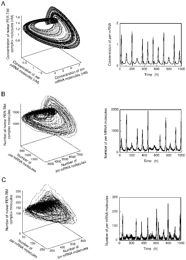
Effect of molecular noise on autonomous chaos. The strange attractor and the corresponding chaotic oscillations predicted by the deterministic PER–TIM model for circadian rhythms are represented in (A). (B) and (C) Progressive dissolution of the strange attractor (left panels) and corresponding aperiodic oscillations (right panels) in the presence of molecular noise, for $Ω = 1000$ and 100, respectively. The curves in (A) are obtained by numerical integration of equations (A.1) listed in Appendix A. In (B) and (C), the curves are obtained by means of the Gillespie algorithm applied to the model of Table 1 in Appendix A. Parameter values are given in Appendix A.

The results indicate that chaos persists in the presence of noise, but the structure of the strange attractor begins to be blurred when the number of molecules decreases and the amplitude of fluctuations rises. Nevertheless the small curler-like substructure that characterises the strange attractor in the PER–TIM model (Fig. 6A, left panel) is still visible in the attractors obtained by stochastic simulations (left panels in Fig. 6B and C).

Because the PER–TIM model can produce periodic as well as chaotic oscillations, we can use this model to compare the effect of molecular noise on the two types of dynamic behaviour. A convenient tool for such a comparison is provided by Poincaré sections. For the case of periodic oscillations, the trajectory in the (M_P, M_T, C_N) plane takes the form of a limit cycle. Intersection of this trajectory with a plane corresponding to a given value of M_T generally yields two points, one for which M_T is on the rise and the other for which M_T is on the decline. Shown in Fig. 7A is the point intersection obtained for the deterministic model when M_T passes the value 1.5 nM upward. Panels B and C in Fig. 7 show the Poincaré sections obtained by stochastic simulations with $Ω = 1000$ and 100, respectively, for the corresponding value of the number of M_T molecules (i.e., 1.5 $Ω$ ). Instead of a single point, we obtain a cloud of points surrounding the deterministic Poincaré section; the smaller the number of molecules, the more scattered the cloud.

Fig. 7
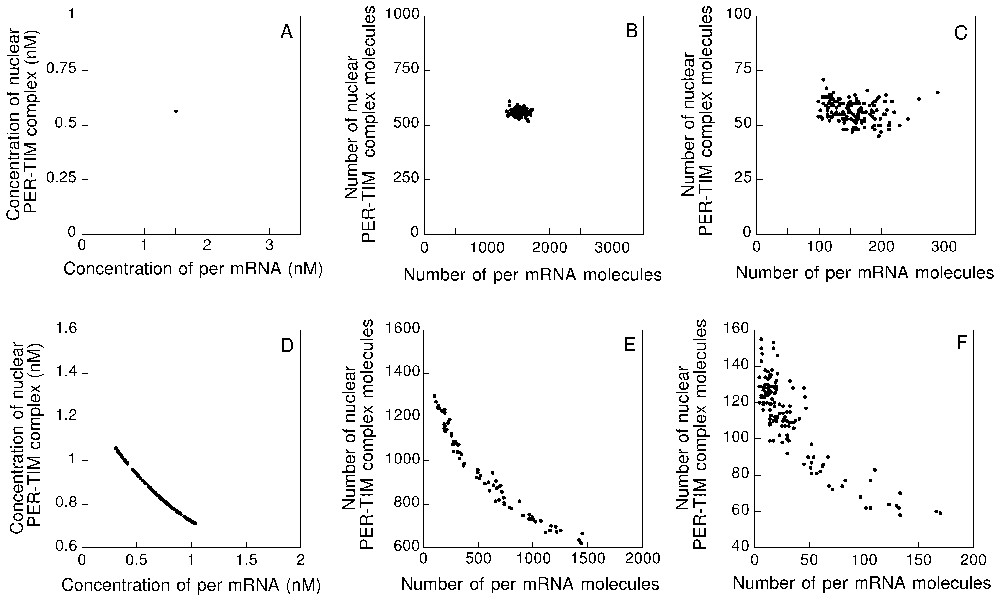
Poincaré sections in the absence or presence of molecular noise. The upper row corresponds to periodic oscillations of the limit cycle type in the deterministic model (A) and in the stochastic model for $Ω = 1000$ (B) and 100 (C) (see corresponding panels in Fig. 2). The bottom row shows the Poincaré sections obtained for chaos in the deterministic model (D) and in the presence of molecular noise for $Ω = 1000$ (E) and 100 (F); these curves correspond, respectively, to panels A–C in Fig. 6. In (A), the section is made when the trajectory crosses the value M_T=1.5 nM upward. In (D), the section corresponds to the upward crossing of the value M_T=5.5 nM. For panels (B) and (C), and (E) and (F), the section corresponds, respectively, to the upward crossing of the value $M_{T} = 1.5 Ω$ and $5.5 Ω$ .

In the case of chaos, instead of a single point the intersection in the deterministic model takes the form of an open continuous curve (Fig. 7D). Stochastic simulations produce a cloudy version of this curve; the scattering of the points in this cloud increases as the number of molecules decreases (compare panels E and F in Fig. 7). Interestingly, in Fig. 7F, we can observe a denser part of the cloud in the left upper part of the figure; this dense region corresponds to noise-induced visits to the curler-like sub-region of the strange attractor (see Fig. 6, left panels).

6 Discussion

Circadian rhythms originate from the negative autoregulation of gene expression. Models based on such regulatory processes have been proposed for circadian rhythms in Drosophila and Neurospora. These models are of a deterministic nature. When molecular noise becomes significant, however, the question arises as to whether genetic control mechanisms can give rise to coherent circadian oscillations at the cellular level. In the presence of reduced numbers of molecules of the mRNA and protein species involved in the circadian clock mechanism, stochastic simulations are needed to address this issue. In a previous publication [17], we studied the stochastic version of a core model for circadian oscillations based on negative autoregulation of a clock gene by its protein product. For stochastic simulations, this deterministic five-variable model was first decomposed into a series of 30 elementary reaction steps. Stochastic simulations performed by means of the Gillespie method [18,19] indicated that robust circadian oscillations, comparable to those predicted by the deterministic approach, can occur in this developed stochastic model even when the maximum numbers of mRNA and clock protein molecules are in the tens and hundreds, respectively. The robustness of circadian rhythms, quantified by the period distribution and the half-time of the autocorrelation function [17], is enhanced when the cooperativity of the repression process increases and when the numbers of mRNA and protein molecules involved in the oscillatory mechanism become larger. Formation of complexes between regulatory proteins is another stabilising factor (D. Forger and C. Peskin, personal communication). Stochastic simulations indicate, moreover, that forcing by a light-dark cycle stabilises the phase of the oscillations [17].

In a follow up study [20] we compared two stochastic versions of the core model for circadian oscillations. In one version (the developed stochastic model), described above, all reactions were decomposed into elementary steps, while in the second version (non-developed model), the reactions were not decomposed into elementary steps and non-linear rate expressions were simply included in the probability of occurrence of each reaction. A comparison of the two stochastic versions of the core model indicates that they both yield similar results; the two approaches are equivalent and corroborate the predictions of the deterministic model. It is only when the maximum numbers of mRNA and protein molecules are reduced to very low values, of the order of a few tens, that molecular noise begins to prevent the emergence of coherent circadian oscillations. These numerical results are corroborated by a recent analytical study [28].

Here we have extended the comparison of deterministic and stochastic models for circadian rhythms by considering a more extended molecular model proposed for circadian oscillations of the PER and TIM proteins and their mRNAs in Drosophila. The ten-variable model is based on the negative autoregulation of the per and tim genes by a complex between the PER and TIM proteins. Although additional proteins are known to be at work in the molecular mechanism of the circadian clock in Drosophila and mammals, the PER–TIM model appears as more realistic than the core mechanism that we previously considered for deterministic [9] and stochastic simulations [17]. Because the non-developed and developed stochastic versions of the core model for circadian rhythms gave similar results, we focused here on the comparison of the deterministic PER–TIM model with its non-developed stochastic version, which is easier to handle than the developed one. An advantage of the PER–TIM model is that, in addition to periodic oscillations, it also admits, for appropriate parameter values, chaotic behaviour. This allowed us to assess the effect of molecular noise both on periodic and chaotic oscillations.

Stochastic simulations of the PER–TIM model corroborate the conclusions reached for the simpler core mechanism for circadian rhythms. Sustained circadian oscillations predicted by the deterministic model are recovered by stochastic simulations. Robust circadian oscillations closely related to those obtained with the deterministic model can already occur when the maximum numbers of protein and mRNA molecules are in the hundreds or tens, respectively (the mean numbers of these molecules in the course of oscillations are smaller, because the levels of both protein and mRNA can go down to very low values at the trough of the oscillations). Robustness increases with the numbers of molecules involved, as reflected by the period distribution (see the period histograms in Fig. 2). It is only at very low numbers of molecules of protein and mRNA (reached, for example, for $Ω = 10$ ) that noise begins to obliterate circadian rhythmicity [17]. In both the deterministic and stochastic versions of the PER–TIM model, critical parameter values separate the evolution toward a stable steady state from the evolution toward sustained oscillations. The effect of noise is merely to induce fluctuations around the stable steady state or around the stable limit cycle predicted by the deterministic model. As shown here (see Fig. 5), and elsewhere on the core model [20], the effect of molecular noise is enhanced in the vicinity of a bifurcation point.

A previous study of models based on negative autoregulation of gene expression reported a lack of robustness of circadian oscillations with respect to molecular noise [16]. The difference with respect to the results presented here and elsewhere [17,20] is likely due to the lower values considered for bimolecular rate constants characterising the association of the repressor to the gene promoter [17,29]. When these parameter values remain too small, the analysis of the deterministic model indicates that the steady state becomes stable but displays the property of excitability: in the stochastic model, instead of sustained oscillations, fluctuations give then rise to irregular, large-amplitude excursions away from the stable steady state.

Autonomous chaos has previously been described in the deterministic PER–TIM model for circadian rhythms in Drosophila [21]. As for periodic circadian oscillations, chaotic behaviour is recovered when stochastic simulations are performed for parameter values corresponding to chaos in the deterministic model. Beyond a noisy appearance due to fluctuations in the presence of reduced numbers of mRNA and protein molecules, the structure of the strange attractor remains discernible (Fig. 6), in agreement with results obtained in models for chemical oscillations [30,31]. The use of Poincaré sections (Fig. 7) allowed us to place on firmer ground the comparison of periodic and chaotic behaviour in the presence of molecular noise. The results lead to a clear distinction between noisy limit cycle oscillations and chaotic oscillations subjected to noise. The agreement between the stochastic and deterministic approaches therefore holds for periodic oscillations as well as for chaotic behaviour.

Acknowledgements

This work was supported by Grant No. 3.4607.99 from the Fonds de la recherche scientifique médicale (FRSM, Belgium). J.-C.L. is Chargé de recherches du FNRS (Belgium). Support from the Fondation David & Alice Van Buuren to D.G. is also acknowledged. We wish to thank F. Baras, G. Dupont, D. Forger, and P. Gaspard for fruitful discussions.

Appendix A

A.0.1 Kinetic equations of the deterministic model for circadian oscillations

The time evolution of the 10 concentration variables in the model of Fig. 1 is governed by the following system of ordinary differential equations: (A.1)

For the case of periodic oscillations in the deterministic model (Figs. 2A and 7A), the following set of parameter values were used: n=4,

v_{sP} = 1.0 nM h^{- 1}

v_{sT} = 1.0 nM h^{- 1}

v_{mP} = 0.7 nM h^{- 1}

v_{mT} = 0.7 nM h^{- 1}

v_{dP} = 2.0 nM h^{- 1}

v_{dT} = 2.0 nM h^{- 1}

, k_sP=k_sT=0.9 h⁻¹, k₁=0.6 h⁻¹, k₂=0.2 h⁻¹,

k_{3} = 1.2 {nM}^{- 1} h^{- 1}

, k₄=0.6 h⁻¹, K_mP=K_mT=0.2 nM, K_IP=K_IT=1.0 nM, K_dP=K_dT=0.2 nM, K_1P=K_1T=K_2P=K_2T=K_3P=K_3T=K_4P=K_4T=2 nM,

V_{1 P} = V_{1 T} = 8 nM h^{- 1}

V_{2 P} = V_{2 T} = 1 nM h^{- 1}

V_{3 P} = V_{3 T} = 8 nM h^{- 1}

V_{4 P} = V_{4 T} = 1 nM h^{- 1}

k_{d} = k_{dC} = k_{dN} = 0.01 nM h^{- 1}

. These values were also used for stochastic simulations in Figs. 2B–D and 7B–C. For chaotic behaviour in the deterministic model (Figs. 6A and 7D) and in stochastic simulations (Figs. 6B and C and 7E and F), the same parameter values were considered, except

v_{mT} = 0.35 nM h^{- 1}

v_{dT} = 5.3 nM h^{- 1}

A.0.2 Stochastic version of the model for circadian oscillations

For stochastic simulations, the model schematised in Fig. 1 and governed by the deterministic system of equations (A.1) is presented as a sequence of reaction steps in Table 1. Steps (21) to (30) refer to non-specific degradation reactions, of relatively reduced importance, which are not indicated in Fig. 1. The second column in Table 1 lists the sequence of reactions (see section 2.2). The probability of each reaction is given in the third column. Parameter values are the same as those listed above for the deterministic model, but units of nM have to be replaced by numbers of molecules, after multiplication of the parameter by $Ω$ , if need be, as indicated in the last column of Table 1.

Bibliographie

[1] M.C. Moore-Ede; F.M. Sulzman; C.A. Fuller The Clocks that Time Us. Physiology of the Circadian Timing System, Harvard University Press, Cambridge, MA, USA, 1982

[2] L.N. Edmunds Cellular and Molecular Bases of Biological Clocks. Models and Mechanisms for Circadian Timekeeping, Springer, New York, 1988

[3] J.C. Dunlap Molecular bases for circadian clocks, Cell, Volume 96 (1999), pp. 271-290

[4] M.W. Young Life's 24-hour clock: molecular control of circadian rhythms in animal cells, Trends Biochem. Sci., Volume 25 (2000), pp. 601-606

[5] J.A. Williams; A. Sehgal Molecular components of the circadian system in Drosophila, Annu. Rev. Physiol., Volume 63 (2001), pp. 729-755

[6] M.W. Young; S.A. Kay Time zones: a comparative genetics of circadian clocks, Nature Rev. Genet., Volume 2 (2001), pp. 702-715

[7] S.M. Reppert; D.R. Weaver Molecular analysis of mammalian circadian rhythms, Annu. Rev. Physiol., Volume 63 (2001), pp. 647-676

[8] P.E. Hardin; J.C. Hall; M. Rosbash Feedback of the Drosophila period gene product on circadian cycling of its messenger RNA levels, Nature, Volume 343 (1990), pp. 536-540

[9] A. Goldbeter A model for circadian oscillations in the Drosophila period protein (PER), Proc. R. Soc. Lond. B, Volume 261 (1995), pp. 319-324

[10] A. Goldbeter Biochemical Oscillations and Cellular Rhythms. The Molecular Bases of Periodic and Chaotic Behaviour, Cambridge University Press, Cambridge, UK, 1996

[11] J.-C. Leloup; A. Goldbeter A model for circadian rhythms in Drosophila incorporating the formation of a complex between the PER and TIM proteins, J. Biol. Rhythms, Volume 13 (1998), pp. 70-87

[12] J.-C. Leloup; D. Gonze; A. Goldbeter Limit cycle models for circadian rhythms based on transcriptional regulation in Drosophila and Neurospora, J. Biol. Rhythms, Volume 14 (1999), pp. 433-448

[13] J.-C. Leloup; A. Goldbeter Modeling the molecular regulatory mechanism of circadian rhythms in Drosophila, BioEssays, Volume 22 (2000), pp. 84-93

[14] H.R. Ueda; M. Hagiwara; H. Kitano Robust oscillations within the interlocked feedback model of Drosophila circadian rhythm, J. Theor. Biol., Volume 210 (2001), pp. 401-406

[15] P. Smolen; D.A. Baxter; J.H. Byrne Modeling circadian oscillations with interlocking positive and negative feedback loops, J. Neurosci., Volume 21 (2001), pp. 6644-6656

[16] N. Barkai; S. Leibler Circadian clocks limited by noise, Nature, Volume 403 (2000), pp. 267-268

[17] D. Gonze; J. Halloy; A. Goldbeter Robustness of circadian rhythms with respect to molecular noise, Proc. Natl Acad. Sci. USA, Volume 99 (2002), pp. 673-678

[18] D.T. Gillespie A general method for numerically simulating the stochastic time evolution of coupled chemical reactions, J. Comput. Phys., Volume 22 (1976), pp. 403-434

[19] D.T. Gillespie Exact stochastic simulation of coupled chemical reactions, J. Phys. Chem., Volume 81 (1977), pp. 2340-2361

[20] D. Gonze; J. Halloy; A. Goldbeter Deterministic versus stochastic models for circadian rhythms, J. Biol. Phys., Volume 28 (2002), pp. 637-653

[21] J.-C. Leloup; A. Goldbeter Chaos and birhythmicity in a model for circadian oscillations of the PER and TIM proteins in Drosophila, J. Theor. Biol., Volume 198 (1999), pp. 445-459

[22] G. Nicolis; I. Prigogine Self-Organization in Nonequilibrium Systems, Wiley, New York, 1977

[23] C.J. Morton-Firth; D. Bray Predicting temporal fluctuations in an intracellular signalling pathway, J. Theor. Biol., Volume 192 (1998), pp. 117-128

[24] F. Baras; J.E. Pearson; M. Malek Mansour Microscopic simulation of chemical oscillations in homogeneous systems, J. Chem. Phys., Volume 93 (1990), pp. 5747-5750

[25] F. Baras Stochastic analysis of limit cycle behaviour (L. Schimansky-Geier; T. Poeschel, eds.), Stochastic Dynamics, Lecture Notes in Physics (LNP484), Springer-Verlag, Berlin, 1997, pp. 167-178

[26] H.H. McAdams; A. Arkin Stochastic mechanisms in gene expression, Proc. Natl. Acad. Sci. USA, Volume 94 (1997), pp. 814-819

[27] A. Arkin; J. Ross; H.H. McAdams Stochastic kinetic analysis of developmental pathway bifurcation in phage λ-infected Escherichia coli cells, Genetics, Volume 149 (1998), pp. 1633-1648

[28] D. Gonze; J. Halloy; P. Gaspard Biochemical clocks and molecular noise, theoretical study of robustness factor, J. Chem. Phys., Volume 116 (2002), pp. 10997-11010

[29] P.H. von Hippel; O.G. Berg Facilitated target location in biological systems, J. Biol. Chem., Volume 264 (1989), pp. 675-678

[30] P. Peeters; G. Nicolis Intrinsic fuctuations in chaotic dynamics, Physica A, Volume 188 (1992), pp. 426-435

[31] P. Geysermans; F. Baras Particle simulation of chemical chaos, J. Chem. Phys., Volume 105 (1996), pp. 1402-1408

[32] E.J. Doedel AUTO, A program for automatic bifurcation analysis of autonomous systems, Congr. Num., Volume 30 (1981), pp. 265-284

Commentaires - Politique

Ces articles pourraient vous intéresser

Circadian rhythm and tumour growth

Jean Clairambault; Philippe Michel; Benoît Perthame

C. R. Math (2006)

An inequality for the Perron and Floquet eigenvalues of monotone differential systems and age structured equations

Jean Clairambault; Stéphane Gaubert; Benoît Perthame

C. R. Math (2007)

Cyclic melatonin synchronises the circadian rhythm of feeding activity in Japanese quail, Coturnix c. japonica

Sophie Lumineau; Catherine Guyomarc’h; Berthe Vivien-Roels; ...

C. R. Biol (2002)