Using mathematical models to help understand biological pattern formation

Philip K. Maini

doi:10.1016/j.crvi.2003.05.006

Biological modelling / Biomodélisation

Using mathematical models to help understand biological pattern formation

Présenté par : Pierre Auger

Philip K. Maini ¹

¹ Centre for Mathematical Biology, Mathematical Institute, 24–29 St Giles', Oxford, OX1 3LB, UK

Comptes Rendus. Biologies, Volume 327 (2004) no. 3, pp. 225-234.

Résumé

One of the characteristics of biological systems is their ability to produce and sustain spatial and spatio-temporal pattern. Elucidating the underlying mechanisms responsible for this phenomenon has been the goal of much experimental and theoretical research. This paper illustrates this area of research by presenting some of the mathematical models that have been proposed to account for pattern formation in biology and considering their implications.

Métadonnées

Reçu le : 2003-04-15
Accepté le : 2003-05-23
Publié le : 2004-03-01

PMID

DOI : 10.1016/j.crvi.2003.05.006

Mots clés : self-organisation, cell movement, chemotaxis, coat markings, slime mold

Affiliations des auteurs :

Philip K. Maini ¹

¹ Centre for Mathematical Biology, Mathematical Institute, 24–29 St Giles', Oxford, OX1 3LB, UK

@article{CRBIOL_2004__327_3_225_0,
     author = {Philip K. Maini},
     title = {Using mathematical models to help understand biological pattern formation},
     journal = {Comptes Rendus. Biologies},
     pages = {225--234},
     publisher = {Elsevier},
     volume = {327},
     number = {3},
     year = {2004},
     doi = {10.1016/j.crvi.2003.05.006},
     language = {en},
}

TY  - JOUR
AU  - Philip K. Maini
TI  - Using mathematical models to help understand biological pattern formation
JO  - Comptes Rendus. Biologies
PY  - 2004
SP  - 225
EP  - 234
VL  - 327
IS  - 3
PB  - Elsevier
DO  - 10.1016/j.crvi.2003.05.006
LA  - en
ID  - CRBIOL_2004__327_3_225_0
ER  -

%0 Journal Article
%A Philip K. Maini
%T Using mathematical models to help understand biological pattern formation
%J Comptes Rendus. Biologies
%D 2004
%P 225-234
%V 327
%N 3
%I Elsevier
%R 10.1016/j.crvi.2003.05.006
%G en
%F CRBIOL_2004__327_3_225_0

Philip K. Maini. Using mathematical models to help understand biological pattern formation. Comptes Rendus. Biologies, Volume 327 (2004) no. 3, pp. 225-234. doi : 10.1016/j.crvi.2003.05.006. https://comptes-rendus.academie-sciences.fr/biologies/articles/10.1016/j.crvi.2003.05.006/

Version originale du texte intégral

1 Introduction

One of the most intriguing properties of many dynamical systems is their ability to spontaneously generate spatial and spatio-temporal patterns. These have been well studied in fluid dynamics (for example, Rayleigh–Bernard convection patterns), materials (crystal growth), ecology (formation of herds), to mention only a few examples. In chemistry, the spontaneous generation of propagating fronts, target patterns, spiral waves and toroidal scrolls in the Belousov–Zhabotinsky reaction has been analysed in great detail. In this reaction, bromate ions oxidise malonic acid in the presence of a catalyst, cerium, which has the states Ce³⁺ and Ce⁴⁺. Sustained periodic oscillations are observed in the cerium ions. If, instead, one uses Fe²⁺ as the catalyst, and Fe³⁺ and phenanthroline, the periodic oscillations are visualised as colour changes between reddish-orange and blue (see, for example, [1,2] for a review). Similar types of patterning arise in physiology and one of the most widely-studied and important areas of wave propagation concerns the electrical activity in the heart [3] which stimulates muscle contraction during heart beat.

In developmental biology, a key aim is to understand the mechanisms underlying spatio-temporal pattern formation. Although genes play a crucial role, a study of genetics alone cannot provide a mechanistic understanding of how physical and chemical processes within a developing system conspire to produce the complex spatio-temporal cues to which cells respond and interact. Indeed, this problem extends beyond developmental biology. For example, in tumour formation, one wishes to understand the combined effects of the signalling cues involved in the regulation of cellular processes no longer functioning properly and new signalling cues initiated by the tumour cells. A number of the processes that occur during the formation and spread of tumour cells are also of vital importance in wound healing, where their function is beneficial to the organism.

In these examples, a number of complex mechanical and biochemical processes interact in a highly nonlinear way. Such systems are amenable to mathematical modelling and the role of the modeller is to suggest explanations, based on biologically plausible mechanisms, of observed behaviour and to make experimentally testable predictions.

There are now a vast number of mathematical and computational models proposed to describe pattern formation in a number of different areas, too many to describe in one article. Therefore, by way of illustration, I will focus on pattern formation in development. In such systems, cell fate can be strongly influenced by environmental factors. Therefore, to answer questions on pattern formation, one must really address the issue of how an organism organises the complex spatio-temporal sequence of signalling cues necessary to develop structure in a controlled and coordinated manner. Structure can form as a result of response to chemical signalling, as a consequence of cell–cell interaction, through tissue movement and rearrangement, or most likely, a combination of all three.

This article is based on a lecture given at the summer school in Bedlewo. Its aim was not to provide a comprehensive review of the field, but to provide to a broad audience a flavour of the types of continuum mathematical models that have been proposed to describe pattern formation in biological systems. Section 2 introduces the concept of chemical pre-pattern models, while Section 3 focusses on cell movement models. Coupling model pattern generators is illustrated in Section 4 by way of two examples. Some biological applications are presented in Sections 5 and 6 is devoted to a discussion.

2 Chemical pre-pattern models

The simplest chemical pre-pattern model is that proposed by Wolpert [4] in which a source-sink mechanism, coupled with diffusion and degradation, leads to a spatial gradient in a single chemical. He proposed that this chemical concentration profile provided positional information for cells, which differentiated according to a series of threshold values. Here, the mechanism of setting up the signalling cue is simple, but the response is complex. Alternatively, the pattern formation step may be complicated, but its interpretation simpler, requiring response to only one threshold value. For example, Turing showed that complicated spatial patterns can be generated due to the reaction and diffusion of a number of chemicals [5], a phenomenon now known as diffusion-driven instability. The reaction kinetics he considered were stabilizing and diffusion is, of course, a homogenizing process. Yet combined in the appropriate way, he showed that these two stabilizing influences could conspire to produce an instability resulting in spatially heterogeneous chemical profiles – a spatial pattern. This is an example of an emergent property and is termed diffusion-driven instability, that is, a spatially uniform steady state, linearly stable in the absence of diffusion, becomes linearly unstable in the presence of diffusion. The resultant spatial pattern is said to have occurred via self-organisation.

The simplest model that can give rise to this instability involves two chemicals and takes the form:

\frac{\partial u}{\partial t} = D_{1} \nabla^{2} u + f (u, v)

(1)

\frac{\partial v}{\partial t} = D_{2} \nabla^{2} v + g (u, v)

(2)

where

u (\underline{x}, t)

and

v (\underline{x}, t)

denote the concentrations of the chemicals u and v respectively, at spatial position

\underline{x}

, and time t on a bounded domain with, typically, zero flux boundary conditions. The functions f and g model the reaction kinetics of u and v, respectively (see examples later). Using standard linear theory (see, for example, [1]) it can be shown that a spatially uniform steady state of the above system can undergo diffusion-driven instability if the following conditions hold:

I f_u+g_v<0
II f_ug_v−f_vg_u>0
III $D_{1} g_{v} + D_{2} f_{u} > 2 \sqrt{D_{1} D_{2} (f_{u} g_{v} - f_{v} g_{u})}$

where all the partial derivatives are evaluated at the spatially uniform steady state.

One possible scenario for pattern formation is that in which f_u and g_u are positive, the latter implying that u activates v, while g_v and f_v are negative, so that v inhibits u (see, for example, [6]). Condition I⇒|f_u|<|g_v|, so from III D₁<D₂. That is, the activator diffuses more slowly than the inhibitor. This is an example of the classic property of many self-organising systems, namely short-range activation, long-range inhibition, an idea first introduced by Gierer and Meinhardt [7].

In Turing's original model, f and g were linear so that if the uniform steady state became unstable, then the chemical concentrations would grow exponentially. This, of course, is biologically unrealistic. Since Turing's paper, a number of models have been proposed wherein f and g are nonlinear so that when the uniform steady state becomes unstable it may or may not evolve to a bounded, stationary, spatially non-uniform, steady state (a spatial pattern) depending on the nonlinear terms. Examples include:

(i) the Gierer–Meinhardt model [7]:
$f (u, v) = α - β u + \frac{γ u^{2}}{v} g (u, v) = δ u^{2} - η v$ (3)
where α,β,γ,δ and η are positive constants, u activates v and v inhibits u;
(ii) the Thomas model [8]:
$f (u, v) = α (u_{0} - u) - \frac{V_{m} uv}{K_{m} + u + u^{2} / K_{s}} g (u, v) = β (v_{0} - v) - \frac{V_{m} uv}{K_{m} + u + u^{2} / K_{s}}$ (4)
where u₀, v₀, α, β, V_m, K_m and K_s are positive constants;
(iii) the Gray–Scott model [9]:
$f (u, v) = - {uv}^{2} + F (1 - u) g (u, v) = {uv}^{2} - (F + k) v$ (5)
where F and k are positive constants.

Although Turing predicted the phenomenon of diffusion-driven instability in 1952, there were many technical difficulties in observing this phenomenon and it was not until almost 40 years later that it was finally observed, in what is now known as the CIMA (chlorite–iodide–malonic acid starch) reaction [10,11]. In the model proposed for this reaction by Lengyel and Epstein [12],

f (u, v) = k_{1} - u - \frac{4 uv}{1 + u^{2}} g (u, v) = k_{2} (u - \frac{uv}{1 + u^{2}})

(6)

where u, v are the concentrations of iodide and chlorite, respectively, and k₁ and k₂ are positive constants.

For these systems, uniform steady state values for u and v can be determined and the model equations linearised about these steady states. Imposing the conditions I–III above defines the parameter space in which diffusion-driven instability occurs.

In many cases, particularly in one dimension, the results of the linear analysis carry over to the weakly nonlinear case but the fully nonlinear system can only be analysed by numerical simulation. It can be shown that the model exhibits, in one dimension, multiple stable steady states, while in two dimensions there is a further degeneracy. For example, the ability to exhibit stripes or spots depends crucially on the type of nonlinearities present (see, for example, [13,14], and Fig. 1).

Fig. 1
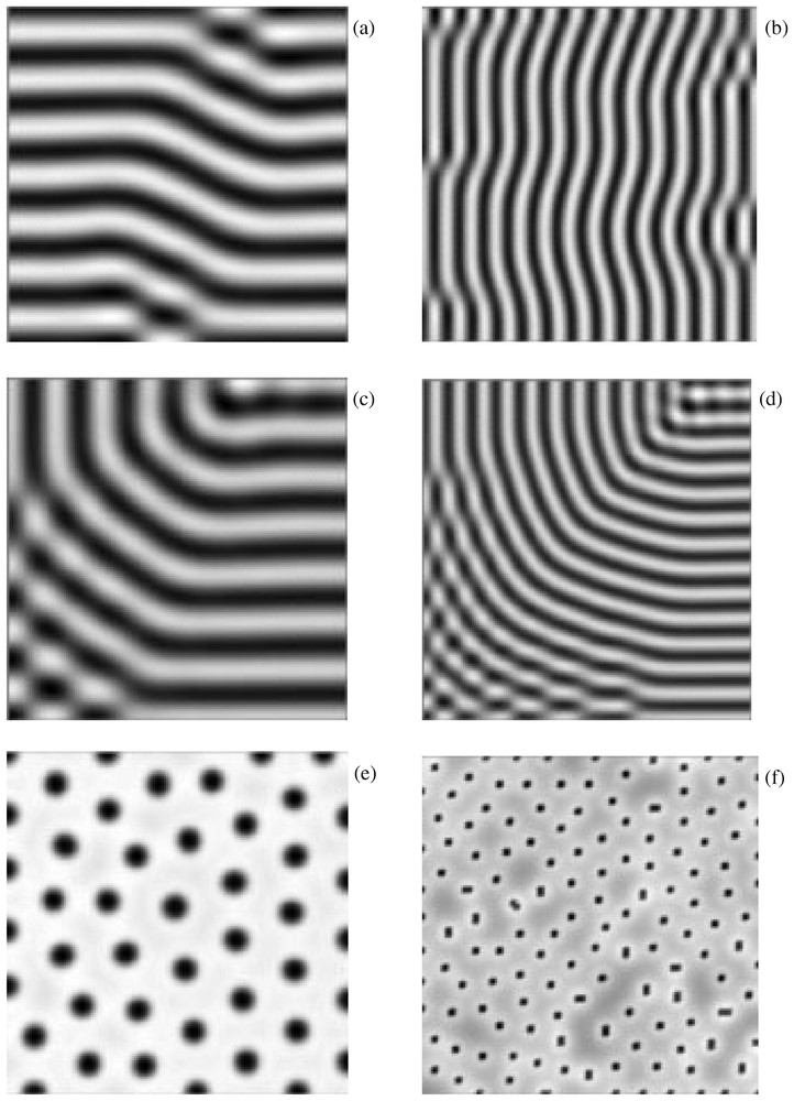
The form of the pattern exhibited by the Turing model in two dimensions depends crucially on the nonlinearity. Spots are favoured by quadratic terms, stripes by cubic terms, after the system has been transformed so that the uniform steady state is (0,0). This is illustrated using the simple kinetics, f(u,v)=αu(1−r₁v²)+v(1−r₂u), $g (u, v) = β v (1 + \frac{α r_{1}}{β} uv) + u (γ + r_{2} v)$ , by choosing the parameters (α, β and γ) in the linear regime so that diffusion-driven instability occurs and then choosing r₁ and r₂ appropriately. (a) r₁=3.5, r₂=0; (b) as in (a) but with α, β and γ chosen to excite a different wavelength solution. By choosing different initial conditions, one can obtain different patterns for the same parameter values, but the spatial scale of the solutions is preserved. This is illustrated by (c) and (d), with parameters as in (a) and (b), respectively. (e) and (f) are the same as (a) and (b), respectively, except that r₁=0.02, r₂=0.2, so that spots are favoured. Reproduced from [15] with permission.

The Gierer–Meinhardt model can exhibit highly localised patterns, known as spike-type solutions. Simplified versions of this model can be analysed to study the dynamics of the spike solutions on one- and two-dimensional domains (see, for example, [16]). This type of behaviour has been observed in the Gray–Scott model and analysed in detail (see, for example, [17,18]). The latter model also exhibits the phenomenon of self-replicating spots, which has been observed experimentally (see, for example, [17,19,20]), and travelling pulses (see, for example, [21]).

There is now a great deal of literature on this subject and general results on the patterning properties of reaction–diffusion equations can be found in the paper by Cross and Hohenberg [22] and the books by Britton [23], Fife [24], Grindrod [25], Murray [1] and Segel [26].

3 Cell movement models

These models describe how cell aggregations can occur spontaneously from an initially spatially homogeneous cell density profile. Essentially, the spatially uniform steady state becomes unstable when the cell dispersing factors (for example, diffusion) are overcome by aggregating factors such as movement up chemical gradients (known as chemotaxis) or adhesive gradients (haptotaxis), or passive convection arising as the result of cell-traction induced deformation of the extracellular matrix (ECM) on which cells move.

The typical chemotaxis model takes the form:

\frac{\partial n}{\partial t} = D_{n} \nabla^{2} n - \nabla \cdot (χ (u) n \nabla u) + f (n, u)

(7)

\frac{\partial u}{\partial t} = D_{u} \nabla^{2} u + g (n, u)

(8)

where

n (\underline{x}, t)

u (\underline{x}, t)

denote cell density and chemoattractant concentration, respectively, at position

\underline{x}

and time t; D_n, D_u are diffusion coefficients, f,g are terms incorporating production and degradation and χ(u) is the chemotactic sensitivity. The latter varies depending on the mode of cell-chemoattractant interaction [27]. This model has been analysed extensively (see, for example, [28,29]) and shown to exhibit bounded spatial patterns. It can also exhibit the phenomena of blow-up and of collapse [27].

Oster et al. [30] showed how mechanical effects could be taken into account. Their model took the form:

\frac{\partial n}{\partial t} = D \nabla^{2} n - α \nabla \cdot (n \nabla ρ) - \nabla \cdot (n \frac{\partial u}{\partial t}) + rn (N - n)

(9)

\frac{\partial ρ}{\partial t} = - \nabla \cdot (ρ \frac{\partial u}{\partial t})

(10)

for the cell and matrix densities,

n (\underline{x}, t)

and

ρ (\underline{x}, t)

, respectively, where D is the diffusion coefficient, α, the haptotactic coefficent, and r and N are constants describing cell production due to logistic growth. Both cell and matrix are assumed to move also by advection, where

u (\underline{x}, t)

is the displacement of a material point of matrix initially at

\underline{x}

They further modelled the ECM as a viscoelastic material at low Reynolds number, so

\nabla \cdot σ + s ρ u = 0

(11)

where

s ρ u

accounts for body forces (modelled as a linear spring where s is the modulus of elasticity of the substrate to which the composite ECM-cell milieu is attached) and σ is the composite stress tensor given by

σ = σ_{ρ} + σ_{n}

(12)

Here σ_ρ is the usual viscoelastic stress tensor

σ_{ρ} = \underset{viscous}{\underset{︸}{μ_{1} \frac{\partial ϵ}{\partial t} + μ_{2} \frac{\partial θ}{\partial t} I}} + \underset{elastic}{\underset{︸}{\frac{E}{1 + ν} (ϵ + \frac{ν}{1 - 2 ν} θ I)}}

(13)

where

θ = \nabla \cdot u

is the dilatation,

ϵ = \frac{1}{2} [\nabla u + \nabla u^{T}]

is the strain tensor,

I

is the unit tensor, μ₁, μ₂ are the shear and bulk viscosities, respectively, and E, ν are the Young's modulus and the Poisson ratio, respectively.

The stress due to cell traction is modelled by

σ_{n} = \frac{τ n ρ}{1 + λ n} I

(14)

where τ and λ are positive constants. This satisfies the conditions that there is no traction without matrix and that traction per cell decreases with increasing cell density (contact inhibition).

Linear and nonlinear analyses, plus numerical simulation, show that models within this general mechanical framework can exhibit steady state spatial patterns [31] and spatio-temporal patterns [32].

4 Coupling pattern generators

The above models provide a framework upon which one can build more complicated and realistic models. For example, it is probable that cells respond to more than one chemotactic cue. Recently, Painter et al. [33] considered the case where the cells respond to two chemical cues, assuming that the latter were components in a Turing system. The simplest such model takes the form:

\frac{\partial u}{\partial t} = D_{1} \nabla^{2} u + f (u, v)

(15)

\frac{\partial v}{\partial t} = D_{2} \nabla^{2} v + g (u, v)

(16)

\frac{\partial n}{\partial t} = D_{n} \nabla^{2} n - \nabla \cdot (χ_{u} (u, v) n \nabla u) - \nabla \cdot (χ_{v} (u, v) n \nabla v)

(17)

where u and v are the chemical concentrations, n the cell density and χ_u(u,v) and χ_v(u,v) are chemotactic sensitivity functions. It is well known that, at primary bifurcation points, the turning points of the chemical concentration profiles in the Turing model coincide. Now, if we consider the above system in one dimension (for simplicity), we have that, at steady state

D_{n} \frac{d n}{d x} = n (χ_{u} \frac{d u}{d x} + χ_{v} \frac{d v}{d x})

(18)

assuming zero flux boundary conditions. Therefore, not only does n have turning points coincident with those of u and v but also, for appropriate χ_u and χ_v, there may be other turning points of n, leading to very complex spatial patterns.

Reaction–diffusion models can have instabilities other than the Turing instability that we have thus far discussed. For example, depending on the nature of the intersection of the nullclines f=g=0 in Eqs. (1) and (2), with D₁=D₂=0, one may obtain excitable behaviour, that is, for extra-threshold stimulation away from the stable steady state, the system undergoes a long excursion before returning to its steady state; it is also possible to obtain oscillatory behaviour. With diffusion included, this leads to the possibility of travelling wavetrain solutions. If one now couples chemotaxis to this system it is possible to obtain a completely different mode of aggregation to that previously described. Cell streaming in the cellular slime mould Dictyostelium discoideum is one such example. This serves as an excellent model paradigm for morphogenesis as it exhibits the processes of signal transduction, signal relay, cell movement and aggregation, all of which play important roles in early embryonic development in higher organisms. Briefly, starvation conditions trigger a developmental programme which is initiated by cell–cell signalling via the extracellular messenger cyclic 3′5′-adenosine monophosphate (cAMP). The chemotactic response to this signal leads to the formation of a multicellular organism composed typically of 10⁴–10⁵ cells. This organism passes through an intermediate motile (slug) phase during which cells differentiate into pre-spore and pre-stalk types, before developing a fruiting body, aiding the dispersal of spores from which, under favourable conditions, new amoebae develop.

Several models have been proposed to account for many of the afore-mentioned phenomena. Here, we focus only on a model for cell aggregation proposed by Höfer et al. [34,35] – we refer the reader to this paper for a fuller description of the biology and parameter values, as well as references to other models. The model takes the form:

\frac{\partial n}{\partial t} = \nabla \cdot (μ \nabla n - χ (v) n \nabla u)

(19)

\frac{\partial u}{\partial t} = λ [ϕ (n) f_{1} (u, v) - (ϕ (n) + δ) f_{2} (u)] + \nabla^{2} u

(20)

\frac{\partial v}{\partial t} = - g (u) v + α (u) (1 - v)

(21)

where n, u and v denote cell density, extracellular cAMP concentration and fraction of active cAMP receptors, respectively.

The second and third equations are a simplified model of the cAMP-cell receptor dynamics (see [36] for full details) modified by cell density effects; the rate of cAMP synthesis per cell is f₁(u,v)=(bv+v²)(a+u²)/(1+u²), where a and b are positive constants. This models autocatalytic production with saturation, mediated by receptor binding. The functions f₂ and g are assumed to be linear in u, to model linear degradation of cAMP and binding of active receptors to cAMP, respectively, while α is assumed to be a positive constant, accounting for the resensitization of the desensitized fraction of receptors at constant rate. This subsystem exhibits excitable dynamics leading to the formation of spiral waves of cAMP concentration. Cell density effects are modelled by the factor φ(n)=n/(1−ρn/(K+n)), where ρ and K are positive constants. This excitable system is coupled with a chemotaxis equation for cell density, with constant diffusion coefficient μ, and chemotactic sensitivity χ(v)=χ₀v^m/(A^m+v^m), m>1, which accounts for adaptation, where χ₀ and A are positive constants. Hence cells only move in the wavefront, when they have a substantial number of active free receptors. The model thus exhibits the pulsatile movement of cells that is observed experimentally. Note that if χ(v) was a constant, as in the classical cell-chemotaxis model, then the cells would move also in the waveback and end up further away from their signalling neighbours than at the start of the signal.

Using experimentally determined parameter values, the above model captures the key features of the aggregation process (see Fig. 2). The model is consistent with the observation that as streaming proceeds, the wavespeed of the spiral patterns decreases, and thus provides an alternative explanation for this phenomenon, which was previously explained by the assumption that biochemical changes must be occurring in the cell-cAMP system, altering the parameter values. In the above model no such change is required because, as the cells form streams, they alter the conditions through which the cAMP waves are propagating. This is initially equivalent to increasing the excitability of the medium which, in turn, leads to an increase in the rotation frequency of the spiral core. As a result [38] the wavespeed of the spiral patterns decreases.

Fig. 2
Numerical simulation showing cell streaming in Dictyostelium discoideum under the influence of two signalling centres. Upper panel: cell density (upper row) and cAMP concentration (lower row) for a counter-rotating pair of spiral waves. Lower panel: cell density and cAMP concentration for a spiral wave and a periodic pacemaker (period 6 min). Initial conditions for the spiral waves were appropriately broken plane wavefronts. Snapshots taken at 10 min, 40 min and 100 min; colour scale ranging from black for low values to white for high values. See [37] for full details.

5 Applications

Turing was the first to formulate the notion of a chemical morphogen, that is, he hypothesized that cells responded to the concentration of certain chemicals and differentiated accordingly. Recently, a number of morphogens have been discovered, but it is still an open question as to whether their spatial pattern is set up by a Turing mechanism. In some cases, for example, the fruit fly Drosophila, it has been shown that some of the early patterning is definitely not due to a Turing-type mechanism, but is set up due to a complex interaction of gradients.

The book by Murray [1] describes a number of applications of the types of models discussed in this paper. Meinhardt [39] has shown that Turing-type models (with two or more chemicals) can exhibit the spectacular variety of patterns seen on sea shells, while Nijhout [40] has shown that such models, together with a small number of sources and sinks, can exhibit the vast array of pigmentation patterns observed on certain butterfly wings. This work has recently been extended (see [41], and Fig. 3).

Fig. 3
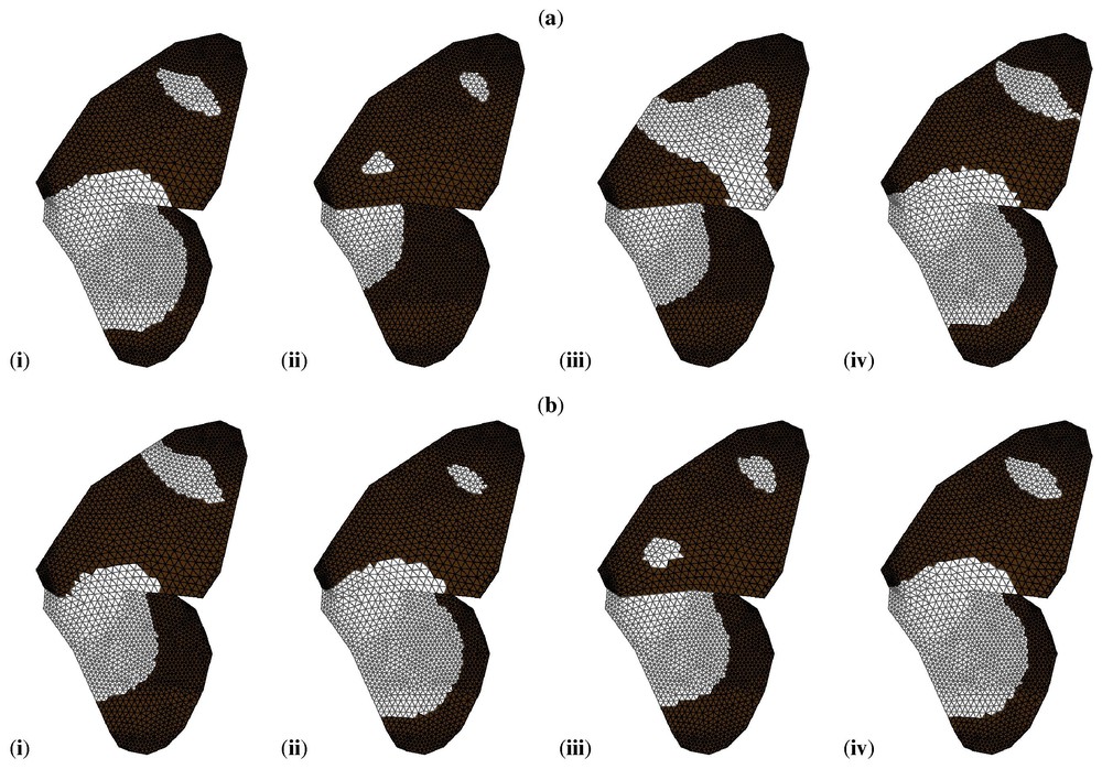
Simulations of the Gierer–Meinhardt model on a geometrically accurate representation of the wing of Papilio dardanus. By varying only a small number of parameters it is possible to reproduce the range of patterns seen in the different mimetic (a) and non-mimetic (b) forms of this butterfly. Black indicates concentrations of v above the threshold value, white indicates concentrations below the threshold. For full details, see [41]. Reproduced from [41] with permission.

These models have been applied to account for animal coat markings [42–46] and to skeletal patterning in the limb (see [47] for a critical review). The Turing model predicts that the complexity of pattern increases with domain size and this has been observed in the chick limb where an experimental manipulation which increases the limb size results in more digits. Conversely, reduction of domain size should decrease the number of digits and this has also been observed.

6 Discussion

The mathematical models that have been presented above propose different scenarios for biological pattern formation. For example, the mechanical model assumes that cells aggregate and differentiate accordingly, while the Turing model assumes that cell density remains uniform and cells differentiate in response to spatially patterned morphogens. Mathematically, thus far it has not been possible to show that there are certain patterns that one of the models exhibits which the other cannot produce. Thus, from a mathematical viewpoint, it is not possible to distinguish, as yet, between these models. However, one could then say that some patterns, and patterning properties are generic and mechanism-independent, and this leads to the notion of developmental constraints [48].

The models propose different scenarios for pattern formation and, to date, it is a highly controversial issue as to which, if any, of the models is the appropriate one. In most of the above models, pattern formation arises as a bifurcation from an initially spatially homogeneous steady state. However, as recognised by Turing, this rarely happens in an embryo, where certain polarities are inherited maternally and the system evolves from one pattern to another. This idea was used by Maini et al. [49], who considered a Turing model in an environment where a gradient of a third chemical controlled the diffusivity of the chemicals in the Turing system. They showed that such a model gave rise to results that were consistent with certain recombination experiments in chick limb that appeared to contradict the Turing model. It turns out that there actually is a gradient in diffusivity across the domain, as hypothesised by the model.

Although the biochemistry underlying the modelling of spatio-temporal patterning in Dictyostelium discoideum is reasonably well known so that models have a firm basis (see [50], and references therein) that is not the case of the other applications presented above. Therefore the issue arises as to whether or not Turing-type instabilities do play a role in biology (as mentioned, they have been shown to occur in chemistry). At the very least, the Turing model, and the subsequent modelling approaches it has inspired, provide a way of thinking about pattern formation that is very different to how it had been thought of before, it increases our intuition, and understanding of the patterning possibilities afforded by combining reaction and diffusion. Moreover, the model equations are arguably some of the richest in mathematics and lead to a number of challenging and fascinating mathematical problems.

Acknowledgements

This paper was written while I was a Foreign Visiting Fellow at the Laboratory of Nonlinear Studies and Computation, Hokkaido University. Sapporo, Japan, and I thank Professor Y. Nishiura for his support and kind hospitality. I acknowledge support from the Royal Society via a Leverhulme Trust Senior Research Fellowship, and thank Ryszard Rudnicki for the invitation to the Summer School at Bedlewo. Finally I thank Thomas Höfer for producing Fig. 2.

Bibliographie

[1] J.D. Murray Mathematical Biology, Springer-Verlag, New York, 1993

[2] B.R. Johnson; S.K. Scott New approaches to chemical patterns, Chem. Soc. Rev., Volume 25 (1996), pp. 265-273

[3] Computational Biology of the Heart (A.V. Panfilov; A.V. Holden, eds.), Wiley, Chichester, UK, 1997

[4] L. Wolpert Positional information and the spatial pattern of cellular differentiation, J. Theor. Biol., Volume 25 (1969), pp. 1-47

[5] A.M. Turing The chemical basis of morphogenesis, Phil. Trans. R. Soc. Lond. B, Volume 327 (1952), pp. 37-72

[6] R. Dillon; P.K. Maini; H.G. Othmer Pattern formation in generalised Turing systems: I. Steady-state patterns in systems with mixed boundary conditions, J. Math. Biol., Volume 32 (1994), pp. 345-393

[7] A. Gierer; H. Meinhardt A theory of biological pattern formation, Kybernetik, Volume 12 (1972), pp. 30-39

[8] D. Thomas Artifical enzyme membranes, transport, memory and oscillatory phenomena (D. Thomas; J.-P. Kernevez, eds.), Analysis and Control of Immobilized Enzyme Systems, Springer, Berlin, 1975, pp. 115-150

[9] P. Gray; S.K. Scott Autocatalytic reactions in the isothermal, continuous stirred tank reactor: oscillations and instabilities in the system A+2B→3B, B→C, Chem. Engrg. Sci., Volume 39 (1984), pp. 1087-1097

[10] V. Castets; E. Dulos; J. Boissonade; P. De Kepper Experimental evidence of a sustained Turing-type equilibrium chemical pattern, Phys. Rev. Lett., Volume 64 (1990), pp. 2953-2956

[11] P. De Kepper; V. Castets; E. Dulos; J. Boissonade Turing-type chemical patterns in the chlorite–iodide–malonic acid reaction, Physica D, Volume 49 (1991), pp. 161-169

[12] I. Lengyel; I.R. Epstein Modeling of Turing structures in the chlorite–iodide–malonic acid-starch reaction system, Science, Volume 251 (1991), pp. 650-652

[13] B. Ermentrout Stripes or spots? Nonlinear effects in bifurcation of reaction–diffusion equations on the square, Proc. R. Soc. Lond. A, Volume 434 (1991), pp. 413-417

[14] B.N. Nagorcka; J.R. Mooney From stripes to spots: prepatterns which can be produced in the skin by a reaction–diffusion system, IMA J. Math. Appl. Med. Biol., Volume 9 (1992), pp. 249-269

[15] R.A. Barrio; C. Varea; J.L. Aragón; P.K. Maini A two-dimensional numerical study of spatial pattern formation in interacting Turing systems, Bull. Math. Biol., Volume 61 (1999), pp. 483-505

[16] M.J. Ward; D. McInerney; P. Houston; D. Gavaghan; P.K. Maini The dynamics and pinning of a spike for a reaction–diffusion system, SIAM J. Appl. Math., Volume 62 (2002), pp. 1297-1328

[17] A. Doelman; T.J. Kappos; P.A. Zegeling Pattern formation in the one-dimensional Gray–Scott model, Nonlinearity, Volume 10 (1997), pp. 523-563

[18] W. Ni Diffusion, cross-diffusion, and their spike-layer steady states, Notices Am. Math. Soc., Volume 45 (1998), pp. 9-18

[19] K.-J. Lee; W.D. McCormick; J.E. Pearson; H.L. Swinney Experimental observation of self-replicating spots in a reaction–diffusion system, Nature, Volume 369 (1994), pp. 215-218

[20] W.N. Reynolds; J.E. Pearson; S. Ponce-Dawson Dynamics of self-replicating patterns in reaction diffusion systems, Phys. Rev. Lett., Volume 72 (1994), pp. 2797-2800

[21] Y. Nishiura; D. Ueyama A skeleton structure of self-replicating dynamics, Physica D, Volume 130 (1999), pp. 73-104

[22] M.C. Cross; P.C. Hohenberg Pattern formation out of equilibrium, Rev. Mod. Phys., Volume 65 (1993), pp. 851-1112

[23] N.F. Britton Reaction–Diffusion Equations and Their Applications to Biology, Academic Press, London, 1986

[24] P. Fife Mathematical Aspects of Reacting and Diffusing Systems, Lect. Notes Biomath., vol. 28, 1979

[25] P. Grindrod The Theory of Applications of Reaction–Diffusion Equations: Pattern and Waves, Oxford University Press, Oxford, UK, 1996

[26] L.A. Segel Modelling Dynamic Phenomena in Molecular and Cellular Biology, Cambridge University Press, Cambridge, UK, 1984

[27] H.G. Othmer; A. Stevens Aggregation, blowup, and collapse: the ABC's of taxis in reinforced random walks, SIAM J. Appl. Math., Volume 57 (1997), pp. 1044-1081

[28] E.F. Keller; L.A. Segel Travelling bands of bacteria: a theoretical analysis, J. Theor. Biol., Volume 30 (1971), pp. 235-248

[29] P.K. Maini; M.R. Myerscough; K.H. Winters; J.D. Murray Bifurcating spatially heterogeneous solutions in a chemotaxis model for biological pattern formation, Bull. Math. Biol., Volume 53 (1991), pp. 701-719

[30] G.F. Oster; J.D. Murray; A.K. Harris Mechanical aspects of mesenchymal morphogenesis, J. Embryol. Exp. Morphol., Volume 78 (1983), pp. 83-125

[31] A.S. Perelson; P.K. Maini; J.D. Murray; J.M. Hyman; G.F. Oster Nonlinear pattern selection in a mechanical model for morphogenesis, J. Math. Biol., Volume 24 (1986), pp. 525-541

[32] G.A. Ngwa; P.K. Maini Spatio-temporal patterns in a mechanical model for mesenchymal morphogenesis, J. Math. Biol., Volume 33 (1995), pp. 489-520

[33] K.J. Painter; P.K. Maini; H.G. Othmer Chemotactic response to multiple signalling cues, J. Math. Biol., Volume 41 (2000), pp. 285-314

[34] T. Höfer; J.A. Sherratt; P.K. Maini Dictyostelium discoideum: cellular self-organization in an excitable biological medium, Proc. R. Soc. Lond. B, Volume 259 (1995), pp. 249-257

[35] T. Höfer; J.A. Sherratt; P.K. Maini Cellular pattern formation during Dictyostelium aggregation, Physica D, Volume 85 (1995), pp. 425-444

[36] J.L. Martiel; A. Goldbeter A model based on receptor desensitization for cyclic AMP signaling in Dictyostelium cells, Biophys. J., Volume 52 (1987), pp. 807-828

[37] T. Höfer, Modelling Dictyostelium aggregation, D.Ph. thesis, Oxford University, 1996

[38] J.J. Tyson; J.P. Keener Singular perturbation theory of traveling waves in excitable media (a review), Physica D, Volume 32 (1988), pp. 327-361

[39] H. Meinhardt The Algorithmic Beauty of Sea Shells, Springer-Verlag, 1995

[40] H.F. Nijhout A comprehensive model for colour pattern formation in butterflies, Proc. R. Soc. Lond. B, Volume 239 (1990), pp. 81-113

[41] T. Sekimura; A. Madzvamuse; A.J. Wathen; P.K. Maini A model for colour pattern formation in the butterfly wing of Papilio dardanus, Proc. R. Soc. Lond. B, Volume 267 (2000), pp. 851-859

[42] J.B.L. Bard A model for generating aspects of zebra and other mammalian coat patterns, J. Theor. Biol., Volume 93 (1981), pp. 363-385

[43] G. Cocho; R. Pérez-Pascual; J.L. Rius Discrete systems, cell–cell interactions and color pattern of animals. I. Conflicting dynamics and pattern formation, J. Theor. Biol., Volume 125 (1987), pp. 419-435

[44] G. Cocho; R. Pérez-Pascual; J.L. Rius; F. Soto Discrete systems, cell–cell interactions and color pattern of animals. I. Clonal theory and cellular automata, J. Theor. Biol., Volume 125 (1987), pp. 437-447

[45] J.D. Murray A pre-pattern formation mechanism for animal coat markings, J. Theor. Biol., Volume 88 (1981), pp. 161-199

[46] J.D. Murray; M.R. Myerscough Pigmentation pattern formation on snakes, J. Theor. Biol., Volume 149 (1991), pp. 339-360

[47] P.K. Maini; M. Solursh Cellular mechanisms of pattern formation in the developing limb, Int. Rev. Cytol., Volume 129 (1991), pp. 91-133

[48] G.F. Oster; J.D. Murray Pattern formation models and development, Zool., Volume 251 (1989), pp. 186-202

[49] P.K. Maini; D.L. Benson; J.A. Sherratt Pattern formation in reaction diffusion models with spatially inhomogeneous diffusion coefficients, IMA J. Math. Appl. Med. Biol., Volume 9 (1992), pp. 197-213

[50] B. Vasiev; C.J. Weijer Modelling Dictystelium Discoideum morphogenesis (P.K. Maini; H.G. Othmer, eds.), Mathematical Models for Biological Pattern Formation, IMA Vol. Math. Appl., vol. 121, Springer-Verlag, 2000, pp. 193-210

Commentaires - Politique

Ces articles pourraient vous intéresser

Complex pattern formation by a self-destabilization of established patterns: chemotactic orientation and phyllotaxis as examples

Hans Meinhardt

C. R. Biol (2003)

Chemotaxis with directional sensing during Dictyostelium aggregation

Rui Dilão; Marcus J.B. Hauser

C. R. Biol (2013)

The biological frontier of pattern formation

Leonid M. Pismen

C. R. Méca (2019)