Travelling-wave analysis of a model of the immune response to cancer

Anastasios Matzavinos; Mark A.J. Chaplain

doi:10.1016/j.crvi.2004.07.016

Biological modelling / Biomodélisation

Travelling-wave analysis of a model of the immune response to cancer
[Analyse de la propagation d'ondes progressives dans un modèle de réponse immunitaire au cancer.]

Présenté par : Pierre Auger

Anastasios Matzavinos ¹ ; Mark A.J. Chaplain ¹

¹ The SIMBIOS Centre, Division of Mathematics, University of Dundee, Dundee, DD1 4HN, UK

Comptes Rendus. Biologies, Volume 327 (2004) no. 11, pp. 995-1008.

Résumés

Anglais
Français

In this paper we present a travelling-wave analysis of a mathematical model describing the growth of a solid tumour in the presence of an immune system response. From a modelling perspective, attention is focused upon the attack of tumour cells by tumour infiltrating cytotoxic lymphocytes (TICLs), in a small multicellular tumour, without necrosis and at some stage prior to (tumour-induced) angiogenesis. As we have shown in previous work, for a particular choice of parameters, the underlying reaction–diffusion–chemotaxis system of partial differential equations is able to simulate the well-documented phenomenon of cancer dormancy by depicting spatially heterogeneous tumour cell distributions that are characterized by a relatively small total number of tumour cells. This behaviour is consistent with several immunomorphological investigations. Moreover, the alteration of certain parameters of the model is enough to induce bifurcations into the system, which in turn result in tumour invasion in the form of a standard travelling wave. The work presented in this paper complements the bifurcation analysis undertaken by Matzavinos et al. [Math. Med. Biol. IMA 21 (2004) 1–34] and establishes the existence of travelling-wave solutions for the system under discussion by promoting the understanding of the geometry of an appropriate phase space.

Dans cet article, nous présentons l'analyse de la propagation d'ondes progressives dans un modèle décrivant la croissance tumorale en présence du système immunitaire. Du point de vue de la modélisation, nous étudions l'attaque des cellules tumorales par des lymphocytes cytotoxiques infiltrants (TICLs) dans une petite tumeur multicellulaire, sans nécrose et à un stade précédent l'angiogenèse (induite par la tumeur). Comme il a été démontré dans un travail antérieur, et pour un choix particulier des paramètres, le système d'équations aux dérivées partielles de réaction–diffusion–chémotaxie permet de simuler le phénomène bien connu de dormance du cancer en présentant des distributions cellulaires hétérogènes dans l'espace caractérisées par un nombre relativement faible de cellules tumorales. Ce comportement est cohérent avec plusieurs résultats immunomorphologiques. De plus, le changement de certains paramètres du modèle est suffisant pour induire des bifurcations du système, qui conduisent à une invasion tumorale sous la forme d'une onde progressive classique. Le travail présenté dans cet article est complémentaire à l'analyse de bifurcations réalisée par Matzavinos (2003) et met en évidence l'existence de solutions de type ondes progressives pour ce système, en donnant des arguments géométriques pour un espace de phase approprié.

Métadonnées

Reçu le : 2004-02-11
Accepté le : 2004-07-29
Publié le : 2004-11-01

PMID

DOI : 10.1016/j.crvi.2004.07.016

Keywords: travelling wave, mathematical modelling, partial differential equations, cancer dormancy, tumour cells, bifurcations
Mot clés : ondes progressives, modélisation mathématique, équations aux dérivées partielles, dormance du cancer, cellules tumorales, bifurcations

Affiliations des auteurs :

Anastasios Matzavinos ¹ ; Mark A.J. Chaplain ¹

¹ The SIMBIOS Centre, Division of Mathematics, University of Dundee, Dundee, DD1 4HN, UK

@article{CRBIOL_2004__327_11_995_0,
     author = {Anastasios Matzavinos and Mark A.J. Chaplain},
     title = {Travelling-wave analysis of a model of the immune response to cancer},
     journal = {Comptes Rendus. Biologies},
     pages = {995--1008},
     publisher = {Elsevier},
     volume = {327},
     number = {11},
     year = {2004},
     doi = {10.1016/j.crvi.2004.07.016},
     language = {en},
}

TY  - JOUR
AU  - Anastasios Matzavinos
AU  - Mark A.J. Chaplain
TI  - Travelling-wave analysis of a model of the immune response to cancer
JO  - Comptes Rendus. Biologies
PY  - 2004
SP  - 995
EP  - 1008
VL  - 327
IS  - 11
PB  - Elsevier
DO  - 10.1016/j.crvi.2004.07.016
LA  - en
ID  - CRBIOL_2004__327_11_995_0
ER  -

%0 Journal Article
%A Anastasios Matzavinos
%A Mark A.J. Chaplain
%T Travelling-wave analysis of a model of the immune response to cancer
%J Comptes Rendus. Biologies
%D 2004
%P 995-1008
%V 327
%N 11
%I Elsevier
%R 10.1016/j.crvi.2004.07.016
%G en
%F CRBIOL_2004__327_11_995_0

Anastasios Matzavinos; Mark A.J. Chaplain. Travelling-wave analysis of a model of the immune response to cancer. Comptes Rendus. Biologies, Volume 327 (2004) no. 11, pp. 995-1008. doi : 10.1016/j.crvi.2004.07.016. https://comptes-rendus.academie-sciences.fr/biologies/articles/10.1016/j.crvi.2004.07.016/

Version originale du texte intégral

1 Introduction

‘Cancer dormancy’ is an operational term used to describe the phenomenon of a prolonged quiescent state in which tumour cells are present, but tumour progression is not clinically apparent [1–3]. As a condition, cancer dormancy is often observed in breast cancers, neuroblastomas, melanomas, osteogenic sarcomas, and in several types of lymphomas, and is often found ‘accidentally’ in tissue samples of healthy individuals who have died suddenly [4,5]. In some cases, cancer dormancy has been found in cancer patients after several years of front-line therapy and clinical remission. The presence of these cancer cells in the body determines, finally, the outcome of the disease. In particular, age, stress factors, infections, act of treatment itself or other alterations in the host can provoke the initiation of uncontrolled growth of initially dormant cancer cells and subsequent waves of metastases [2,6]. Recently, some molecular targets for the induction of cancer dormancy and the re-growth of a dormant tumour have been identified [7,8]. However, the precise nature of the phenomenon remains poorly understood.

One of the main factors (but not the only one) contributing to the induction and maintenance of cancer dormancy is the reaction of the host immune system to the tumour cells [1,2]. Indeed, tumour-associated antigens can be expressed on tumour cells at very early stages of tumour progression [9] and, as a consequence, during the avascular stage, tumour development can be effectively controlled by tumour-infiltrating cytotoxic lymphocytes (TICLs) [10]. The TICLs may be cytotoxic lymphocytes (CD8⁺ CTLs), natural killer-like (NK-like) cells and/or lymphokine activated killer (LAK) cells [11–14].

In [15] we developed a mathematical model for the spatio-temporal response of cytotoxic T-lymphocytes to a solid tumour. For a particular choice of parameters the model was able to simulate the phenomenon of cancer dormancy by depicting spatially unstable and heterogeneous tumour cell distributions that were nonetheless characterized by a relatively small total number of tumour cells. This behaviour was consistent with several immunomorphological investigations. However, the alteration of certain parameters of the model was enough to induce bifurcations into the system, which in turn resulted in the existence of travelling-wave-like solutions in the numerical simulations. These travelling waves were of great importance because when they existed, the tumour invaded the healthy tissue at its full potential escaping the host's immune surveillance.

It is worth mentioning that the cancer dormancy solutions were characterized by an irregular evolution, which according to several objective indications, was an actual manifestation of spatio-temporal chaos. In particular, a bifurcation analysis of the ODE kinetics of our system has revealed the existence of oscillatory solutions for the ODE system emerging through a Hopf bifurcation. We have presented these results in [15] and have indicated several connections with spatio-temporal chaotic systems that couple oscillatory kinetics with diffusion (see, for example, the excellent work on λ–ω systems presented in [16]). Furthermore, we have been able to correlate numerically the existence of the stable limit cycle that emerged through the Hopf bifurcation with the irregular spatio-temporal evolution of the PDE system and the onset of cancer dormancy.

In recent years several papers have begun to investigate the mathematical modelling of the various aspects of the immune system response to cancer. The development of models which reflect several spatial and temporal aspects of tumour immunology can be regarded as the first step towards an effective computational approach in investigating the conditions under which tumour recurrence takes place and in the optimising of both spatial and temporal aspects of the application of various immunotherapies. Key papers in this area include [17–22], which focus on the modelling of tumour progression and immune competition by generalized kinetic (Boltzmann) models and [23–26], which focus on the development of tumour heterogeneities as a result of tumour cell and macrophage interactions. Moreover, [27] is concerned with receptor–ligand (Fas–FasL) dynamics, [28] investigates the process of macrophage infiltration into avascular tumours, [15,29,30] focus on the dynamics of tumour cell–TICL interactions, and finally [31] and [32] analyze various immune system and immunotherapy models in the context of cancer dynamics.

In this paper we undertake a travelling-wave analysis of a sub-system of the model presented in [15]. The full system involved some spatially non-uniform kinetic terms through the introduction of a Heaviside function modelling some aspects of the geometry over which the system was solved. This spatial non-uniformity in the kinetics complicates the travelling-wave analysis and for the sake of mathematical simplicity it is not treated here (see also the comments in [15] concerning the effect that the Heaviside function in the kinetics has on the spatio-temporal simulations). Furthermore, we also do not consider the chemotaxis aspect of the full system. Thus the model under consideration will be a nonlinear reaction–diffusion system of partial differential equations.

2 The mathematical model

For the sake of completeness we first of all introduce the complete model as it has been discussed in [15]. Let us consider a simplified process of a small, growing, avascular tumour which elicits a response from the host immune system and attracts a population of lymphocytes. The growing tumour is directly attacked by TICLs [33–35] which, in turn, secrete soluble diffusible factors (chemokines). These factors enable the TICLs to respond in a chemotactic manner (in addition to random motility) and migrate towards the tumour cells. Our model will therefore consist of six dependent variables denoted E, T, C, $E^{*}$ , $T^{*}$ and α, which are the local densities/concentrations of TICLs, tumour cells, TICL–tumour cell complexes, inactivated TICLs, ‘lethally hit’ (or ‘programmed-for-lysis’) tumour cells, and a single (generic) chemokine, respectively.

The local interactions between the TICLs and tumour cells may be described by the simplified kinetic scheme given in Fig. 1 (see [30] and [15] for full details). The parameters $k_{1}$ , $k_{−1}$ and $k_{2}$ are non-negative kinetic constants: $k_{1}$ and $k_{−1}$ describe the rate of binding of TICLs to tumour cells and detachment of TICLs from tumour cells without damaging cells; $k_{2}$ is the rate of detachment of TICLs from tumour cells, resulting in an irreversible programming of the tumour cells for lysis (i.e. death) with probability p or inactivating/killing TICLs with probability $(1 - p)$ . Using the law of mass action the above kinetic scheme can be ‘translated’ into a system of ordinary differential equations. Furthermore, we consider other kinetic interaction terms between the variables and examine migration mechanisms for the TICLs, tumour cells and also consider diffusion of the chemokines. We assume that there is no ‘nonlinear’ migration of cells and no nonlinear diffusion of chemokine i.e. all random motility, chemotaxis and diffusion coefficients are assumed constant.

Fig. 1
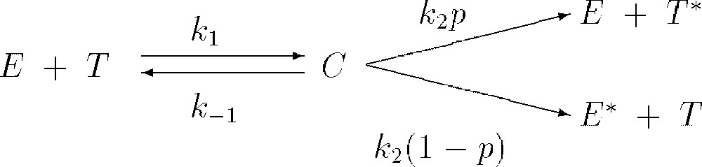
Schematic diagram of local lymphocyte–cancer cell interactions.

We assume that the TICLs have an element of random motility and also respond chemotactically to the chemokines. There is a source term modelling the underlying TICL production by the host immune system, a linear decay (death) term and an additional TICL proliferation term in response to the presence of the tumour cells. Combining these assumptions with the local kinetics (derived from Fig. 1) we have the following PDE for TICLs:

\frac{\partial E}{\partial t} = \overset{random motility}{\overset{︷}{D_{1} \nabla^{2} E}} - \overset{chemotaxis}{\overset{︷}{χ \nabla \cdot (E \nabla α)}} + \overset{supply}{\overset{︷}{s \cdot h (x)}} + \overset{proliferation}{\overset{︷}{\frac{f C}{g + T}}} - \overset{decay}{\overset{︷}{d_{1} E}} - \overset{local kinetics}{\overset{︷}{k_{1} E T + (k_{−1} + k_{2} p) C}}

(1)

where

D_{1}

, χ, s, f, g,

d_{1}

,

k_{1}

,

k_{−1}

,

k_{2}

, p are all positive constants.

D_{1}

is the random motility coefficient of the TICLs and χ is the chemotaxis coefficient. The parameter s represents the ‘normal’ rate of flow of mature lymphocytes into the tissue (non-enhanced by the presence of tumour cells). The function

h (x)

is a Heaviside function, which aims to model the existence of a subregion of the domain of interest where initially there are only tumour cells and where lymphocytes do not reside. This region of the domain is penetrated by effector cells subsequently through the processes of diffusion and chemotaxis only (see [15] for a full discussion regarding this assumption). The proliferation term

f C / (g + T)

represents the experimentally observed enhanced proliferation of TICLs in response to the tumour and has been derived through data fitting [15,30]. This functional form is consistent with a model in which one assumes that the enhanced proliferation of TICLs is due to signals, such as released interleukins, generated by effector cells in tumour cell–TICL complexes. We note that the growth factors that are secreted by lymphocytes in complexes (e.g., IL-2) act mainly in an autocrine fashion. That is to say they act on the cell from which they have been secreted and thus, in our spatial setting, their action can be adequately described by a ‘local’ kinetic term only, without the need to incorporate any additional information concerning diffusivity.

We assume that the chemokines are produced when lymphocytes are activated by tumour cell–TICL interactions. Thus we define chemokine production to be proportional to tumour cell–TICL complex density C. Once produced the chemokines are assumed to diffuse throughout the tissue and to decay in a simple manner with linear decay kinetics. Therefore the PDE for the chemokine concentration is:

\frac{\partial α}{\partial t} = \overset{diffusion}{\overset{︷}{D_{2} \nabla^{2} α}} + \overset{production}{\overset{︷}{k_{3} C}} - \overset{decay}{\overset{︷}{d_{4} α}}

(2)

where

D_{2}, k_{3}, d_{4}

are positive parameters.

We assume that migration of the tumour cells may be described by simple random motility and that on the kinetic level the growth dynamics of a solid tumour may be described adequately by a logistic term (see [15] for a full discussion concerning the validity of these assumptions). Hence the PDE governing the evolution of tumour cell density is:

\frac{\partial T}{\partial t} = \overset{random motility}{\overset{︷}{D_{3} \nabla^{2} T}} + \overset{logistic growth}{\overset{︷}{b_{1} (1 - b_{2} T) T}} - \overset{local kinetics}{\overset{︷}{k_{1} E T + (k_{−1} + k_{2} (1 - p)) C}}

(3)

where

D_{3}

is the random motility coefficient of the tumour cells,

b_{1}

,

b_{2}

,

k_{1}

,

k_{−1}

,

k_{2}

, p are positive parameters.

We assume that there is no diffusion of the complexes, only interactions governed by the local kinetics derived from Fig. 1. The absence of a diffusion term is justified by the fact that formation and dissociation of complexes occurs on a time scale of tens of minutes, whereas the random motility of the tumour cells, for example, occurs on a time scale of tens of hours. Thus, the cell–cell complexes do not have time to move. Therefore the equation for the complexes is given by:

\frac{\partial C}{\partial t} = \overset{local kinetics}{\overset{︷}{k_{1} E T - (k_{−1} + k_{2}) C}}

(4)

We assume that inactivated and ‘lethally hit’ cells (i.e. cells that will die) are quickly eliminated from the tissue (for example, by macrophages) and do not substantially influence the immune processes being analysed. Inactivated cells also do not migrate and therefore we have:

\frac{\partial E^{*}}{\partial t} = \overset{local kinetics}{\overset{︷}{k_{2} (1 - p) C}} - \overset{decay}{\overset{︷}{d_{2} E^{*}}}

(5)

\frac{\partial T^{*}}{\partial t} = \overset{local kinetics}{\overset{︷}{k_{2} p C}} - \overset{decay}{\overset{︷}{d_{3} T^{*}}}

(6)

It is easy to see that Eqs. (5) and (6) are only coupled to the full system through the complexes C and that neither $E^{*}$ nor $T^{*}$ have any effect on the variable C. Thus, Eqs. (1)–(4) essentially dictate the behaviour of the complete system.

The system of Eqs. (1)–(4) is closed by applying appropriate boundary and initial conditions. In the one-dimensional case, we define the spatial domain to be the interval $[0, x_{0}]$ and we assume that there are two distinct regions in this interval – one region entirely occupied by tumour cells, the other entirely occupied by the immune cells. We propose that an initial interval of tumour localization is $[0, l]$ , where $l = 0.2 x_{0}$ . In this framework the function $h (x)$ (cf. Eq. (1)) is defined by:

h (x) = {\begin{matrix} 0, & if x - l ⩽ 0 \\ 1, & if x - l > 0 \end{matrix}

and the initial conditions are given by:

(7)

where

(8)

In addition, zero-flux boundary conditions are imposed on the variables E, α and T. A full discussion of the biological interpretation of the particular initial and boundary conditions can be found in [15].

The closed system is non-dimensionalized by choosing an order-of-magnitude scale for the E, T and C cell densities, of $E_{0}$ , $T_{0}$ and $C_{0}$ , respectively, as suggested by the initial conditions. The chemokine concentration α is normalised through some reference concentration $α_{0}$ discussed in [15]. Time is scaled relative to the diffusion rate of the TICLs, i.e. $t_{0} = x_{0}^{2} D_{1}^{−1}$ and the space variable x is scaled relative to the length of the region under consideration, i.e. $x_{0} = 1 cm$ .

An estimation of the parameters of the system based on experimental data has been obtained in [15]. The experimental data used were concerned with dormant murine B cell lymphomas [2,36]. The corresponding numerical simulations of the non-dimensionalized system with the estimated values for the parameters under discussion were able to reproduce several characteristics of a tumour in its dormant state. Figs. 2a, 3a and 4a show the initial conditions for the TICL, tumour cell and TICL–tumour cell densities, respectively. Fig. 2b–d shows the evolution of the (non-dimensionalized) spatial distribution of TICL density within the tissue at times corresponding to 700, 1000 and 1300 days, respectively. The time instances depicted in the figures show the formation of an unstable, heterogeneous spatial distribution of TICL density throughout the tissue. Fig. 3b–d shows the spatial distribution of tumour cell density within the tissue at times corresponding to 700, 1000 and 1300 days. The figures show a train of solitary-like waves invading the tissue and subsequently creating a spatially heterogeneous distribution of tumour cell density throughout. Fig. 4b–d shows time instances of the corresponding TICL–tumour cell complex distribution at 700, 1000 and 1300 days, respectively.

Fig. 2
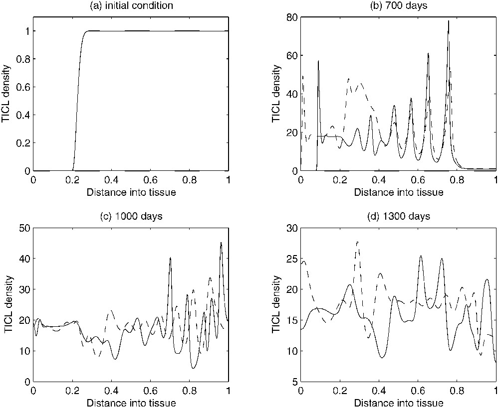
Figures showing plots of the TICL density over time. As time evolves, the complicated spatio-temporal dynamics can be observed. The solid-line curves show results when chemotaxis of the TICLs is incorporated into the system. The dashed line curves show results when there is no chemotaxis (i.e. χ=0), only random motility of TICLs.

Fig. 3
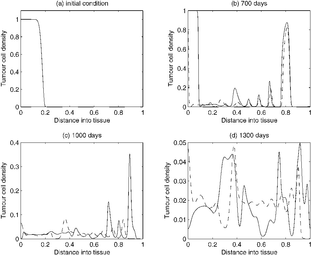
Figures showing plots of the tumour cell density over time. As time evolves, the complicated spatio-temporal dynamics can be observed. The solid-line curves show results when chemotaxis of the TICLs is incorporated into the system. The dashed line curves show results when there is no chemotaxis (i.e. χ=0), only random motility of TICLs.

Fig. 4
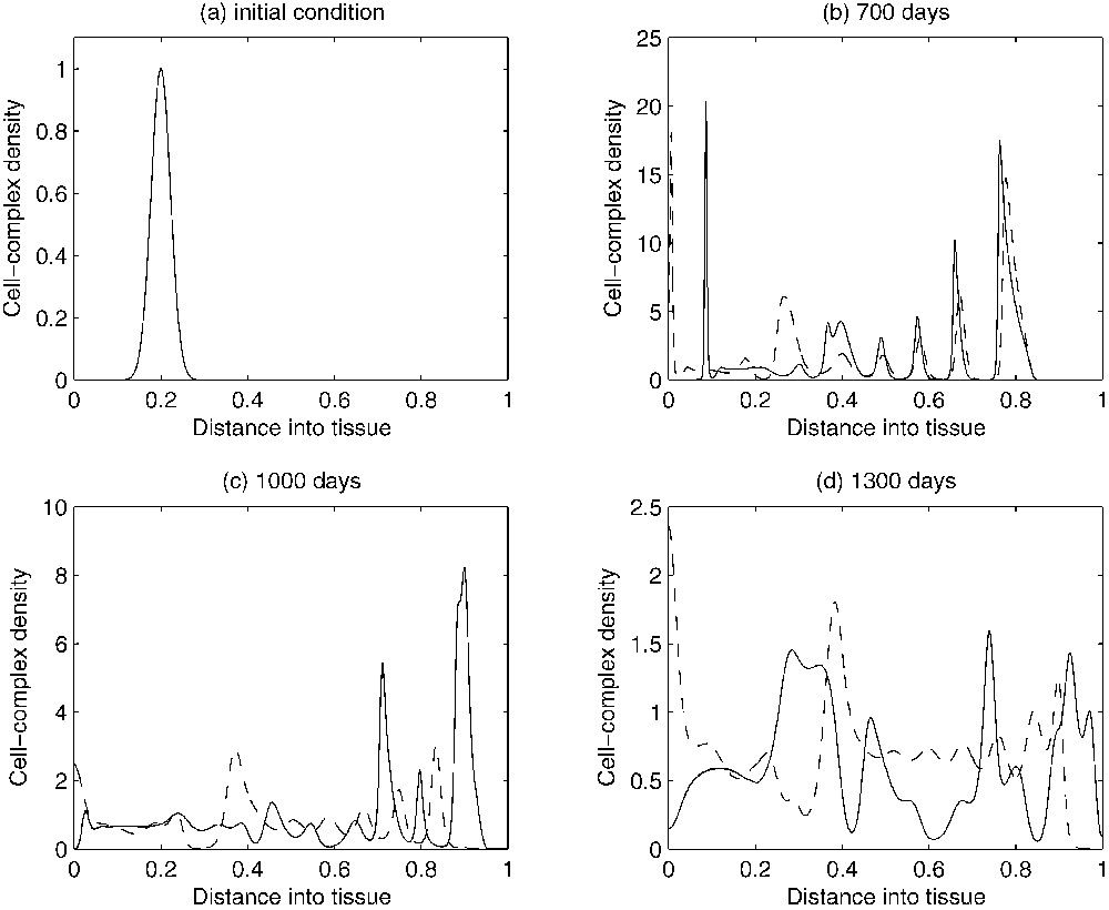
Figures showing plots of the TICL-tumour-cell complex density over time. As time evolves, the complicated spatio-temporal dynamics can be observed. The solid-line curves show results when chemotaxis of the TICLs is incorporated into the system. The dashed line curves show results when there is no chemotaxis (i.e. χ=0), only random motility of TICLs.

In addition to observing the above spatio-temporal distributions of each cell type within the tissue, the temporal dynamics of the overall populations of each cell type (i.e. total cell number) was examined. This was achieved by calculating the total number of each cell type within the whole tissue space using numerical quadrature. Fig. 5a shows the variation in the number of TICLs within the tissue over time (approximately 80 years, an estimated average lifespan). Initially, the total number of TICLs within the tissue increases and then subsequently oscillates around some stationary level (approximately $5.9 \times 10^{6}$ cells). Long-time numerical calculations indicated that this behaviour will persist for all time. A similar scenario is observed for the tumour cell population. From Fig. 5b, we observe that initially, the tumour cell population decreases in number before subsequently oscillating around some stationary value (approximately 10⁷ cells) for all time. Fig. 5c gives the corresponding temporal dynamics of the complexes.

Fig. 5
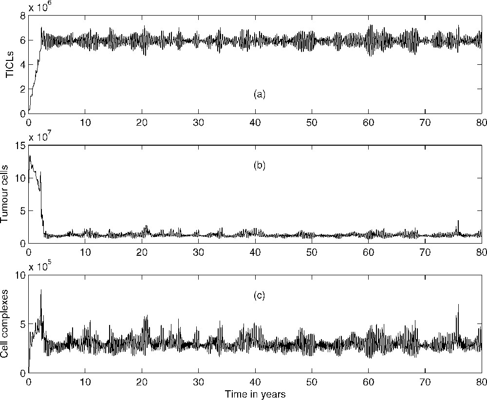
Total number of (a) lymphocytes, (b) tumour cells, and (c) tumour cell–TICL complexes within tissue over a period of 80 years.

In [15] we have been able to correlate numerically the irregular spatio-temporal evolution of the system (1)–(4) depicted in the above simulations with the existence of a stable limit cycle that emerged through a Hopf bifurcation in the spatially homogeneous ODE kinetics. Although the bifurcation analysis presented in [15] is out of the scopes of this article, we would like to correct a previous error by presenting a small (corrected) part of the relevant analysis. In particular, we focus on the bifurcations of the non-dimensionalized homogeneous ODE kinetics of Eqs. (1)–(4) with the Heaviside function omitted (i.e. $h (x) \equiv 1$ ) and with respect to parameter $k_{1}$ , which is crucial in revealing the existence of the Hopf bifurcation under discussion. The bifurcation diagrams presented here have been generated with the version of the AUTO routine that is implemented within the XPP software package [37]. Fig. 6 shows part of the bifurcation diagram of TICL density E versus parameter $k_{1}$ . In the case of our system, AUTO was able to detect a (super-critical) Hopf bifurcation at $k_{1} = 8.421 \times 10^{−8} {day}^{−1} {cells}^{−1} cm$ . The solid dots represent the maximum and minimum values of the periodic solutions that emerge when $k_{1}$ lies in a particular interval. Most of the limit cycles that emerge through this bifurcation, including the one that is generated for $k_{1} = 1.3 \times 10^{−7} {day}^{−1} {cells}^{−1} cm$ (the parameter value that is associated with the irregular spatio-temporal simulations presented here), have been characterized by AUTO as stable. However there is a region around $k_{1} = 1.92 \times 10^{−7} {day}^{−1} {cells}^{−1} cm$ where unstable limit cycles exist. Fig. 7 shows a detailed view of this part of the bifurcation diagram. Here the solid dots represent stable limit cycle solutions, whereas the open circles represent unstable limit cycle solutions. As can be seen we have co-existence of stable and unstable limit cycles. Fig. 8, which has been generated with the MATLAB continuation toolbox MATCONT [38,39], reveals the structure of the projections of the limit cycles emerging at the co-existence region to the $(E, T)$ phase-plane. The existence of a fold or limit-point cycle (LPC) is evident.

Fig. 6
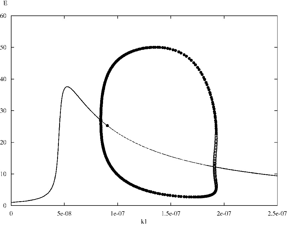
Bifurcation diagram of TICL density E versus the parameter $k_{1}$ .

Fig. 7
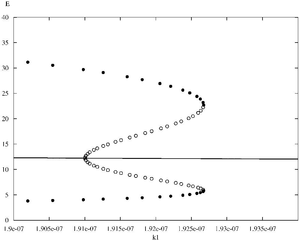
Detailed view of the co-existence region of Fig. 6.

Fig. 8
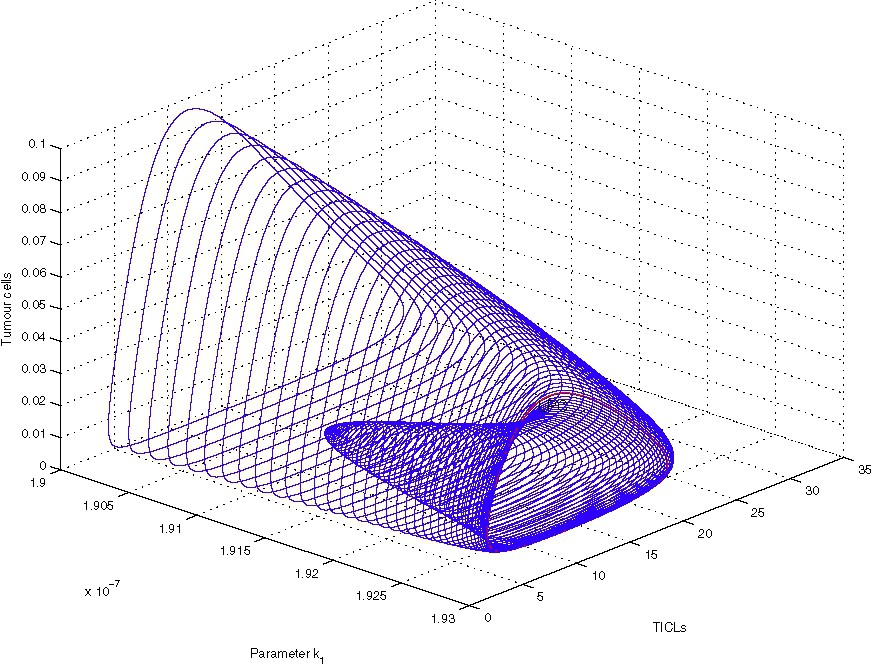
Limit-cycle-projection continuation in the co-existence region.

The above spatio-temporal simulations appear to indicate that eventually the tumour cells develop very small-amplitude oscillations about a ‘dormant’ state, indicating that the TICLs have successfully managed to keep the tumour under control. The numerical simulations demonstrate the existence of cell distributions that are quasi-stationary in time but unstable and heterogeneous in space. However, one would expect that by reducing the probability p of tumour cells being killed by lymphocytes, travelling-wave-like solutions of more canonical nature should emerge. Indeed, reducing the parameter p in the simulations results in the emergence of solutions of a composite type consisting of steady-state and travelling-wave components both in the full system and in the system without chemotaxis (i.e. the system of Eqs. (1), (3) and (4) with $χ = 0$ ). Figs. 9–11 show the evolution of these composite solutions from the initial conditions for the full system (with chemotaxis incorporated).

Fig. 9
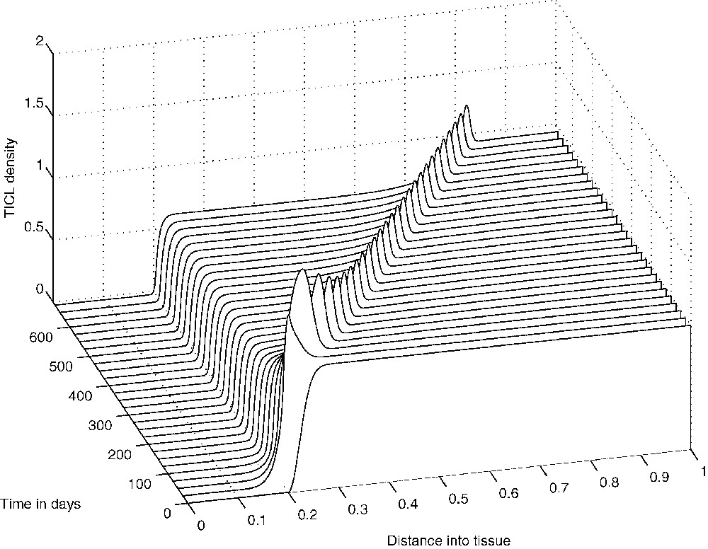
The evolution from the initial conditions of a ‘composite’ solution concerning TICL density E.

Fig. 10
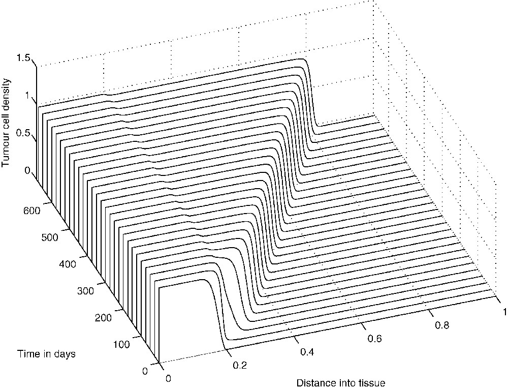
The evolution from the initial conditions of a ‘composite’ solution concerning tumour cell density T.

Fig. 11
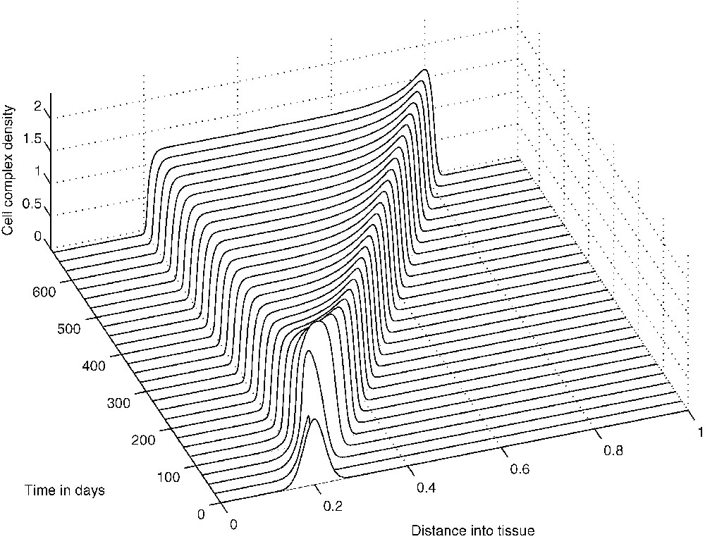
The evolution from the initial conditions of a ‘composite’ solution concerning cell-complex density C.

Our intention in this paper is to investigate the travelling-wave components of the composite solutions that arise for a particular range of values of parameter p (see also the bifurcation analysis undertaken in [15]). For the sake of mathematical simplicity we will not consider the effect of chemotaxis. That is to say we will investigate the solutions of the system of Eqs. (1), (3) and (4) with $χ = 0$ . We would like to note here that this is a reasonable simplifying assumption since, according to the numerical simulations that follow, the formation of the travelling-wave components is not affected by the chemotaxis term. Furthermore, we omit the Heaviside function, i.e. we set $h (x) \equiv 1$ . We note that the Heaviside function is responsible for the formation of the steady-state components of the composite solutions (see also the relevant discussion in [15] concerning the effect that the Heaviside function has on the spatio-temporal simulations) and thus by omitting it we choose to focus on the travelling-wave components. Specifically then, we will focus on the following non-dimensionalized reaction–diffusion system:

\frac{\partial E}{\partial t} = \nabla^{2} E + σ + \frac{ρ C}{η + T} - σ E - μ E T + ɛ C

(9)

\frac{\partial T}{\partial t} = ω \nabla^{2} T + β_{1} (1 - β_{2} T) T - ϕ E T + λ C

(10)

\frac{\partial C}{\partial t} = μ E T - ψ C

(11)

where

σ = \frac{s t_{0}}{E_{0}} = d_{1} t_{0}, ρ = \frac{f t_{0} C_{0}}{E_{0} T_{0}}

μ = \frac{k_{1} t_{0} T_{0} E_{0}}{C_{0}} = k_{1} t_{0} T_{0}, η = \frac{g}{T_{0}}

ɛ = \frac{t_{0} C_{0} (k_{−1} + k_{2} p)}{E_{0}}, ω = \frac{D_{3} t_{0}}{x_{0}^{2}} = D_{3} D_{1}^{−1}

β_{1} = b_{1} t_{0}, β_{2} = b_{2} T_{0}, ϕ = k_{1} t_{0} E_{0}

λ = \frac{t_{0} C_{0} (k_{−1} + k_{2} (1 - p))}{T_{0}}, ψ = t_{0} (k_{−1} + k_{2})

and

E_{0}

,

T_{0}

and

C_{0}

are the order-of-magnitude scales defined by (8). The parameter p affects the non-dimensionalized parameters ɛ and λ and thus the reduction of p leads to different values of ɛ and λ than the ones used in the tumour-dormancy simulations. In what follows we employ the parameter values given in Table 1. These are obtained from the estimated dimensional parameters by reducing the parameter p (see also the relevant bifurcation analysis in [15]). In particular parameter p is here set at 0.99, whereas in the simulation results depicted in Figs. 2–5,

p = 0.9997

.

σ=41 200	ρ=59 760	η=0.0404	μ=6.5×10⁷
ɛ=31 128 000.01	ω=1	$β_{1} = 1.8 \times 10^{5}$	$β_{2} = 1$
ϕ=42 912.6214	λ=15 892.19418	ψ=3.12×10⁷

The system of Eqs. (9), (10) and (11) has been solved numerically over the interval $[0, 1]$ with zero-flux boundary conditions imposed and the initial conditions given by the non-dimensionalization of Eqs. (7). Figs. 12–14 show the results of the numerical simulations, which clearly depict the evolution of standard travelling waves from the initial conditions. We note that these travelling waves – and the corresponding composite solutions of the full system – are of great biological importance because, when they exist, the tumour invades the healthy tissue at its full potential. In the next section we undertake a travelling-wave analysis of system (9)–(11).

Fig. 12
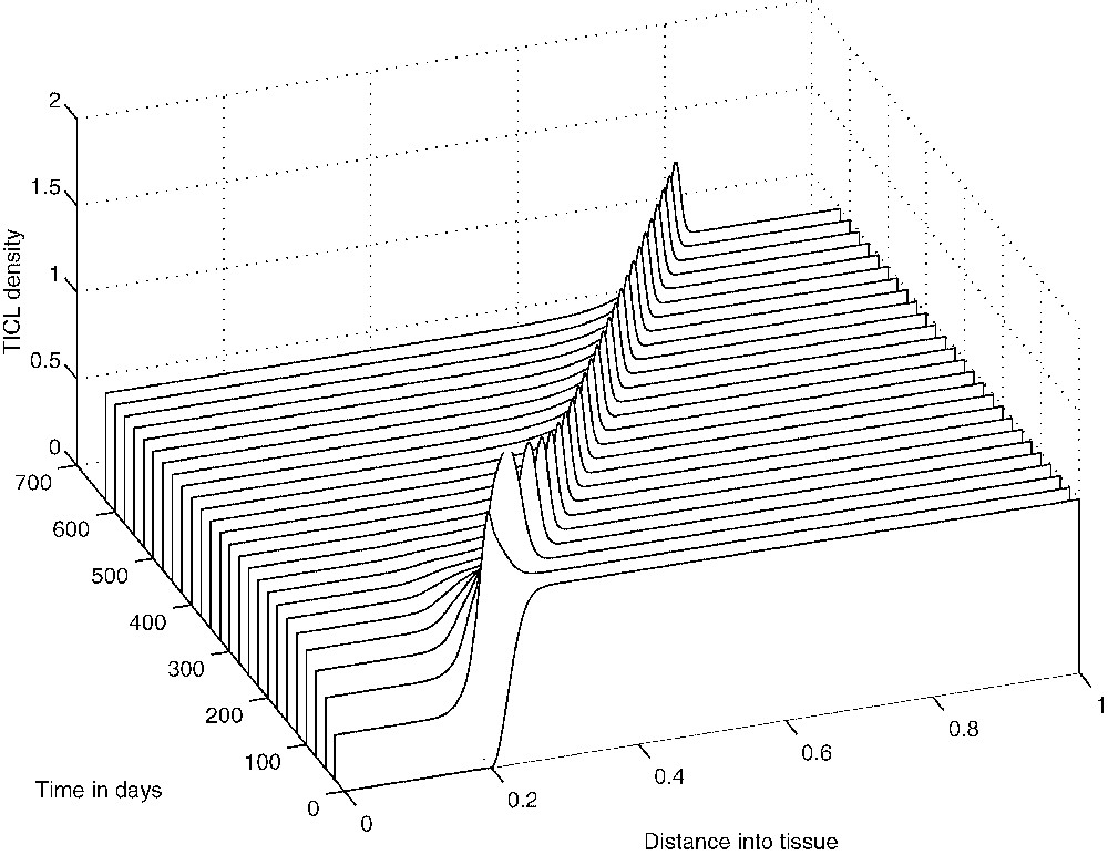
The evolution from the initial conditions of the travelling wave of effector cell density.

Fig. 13
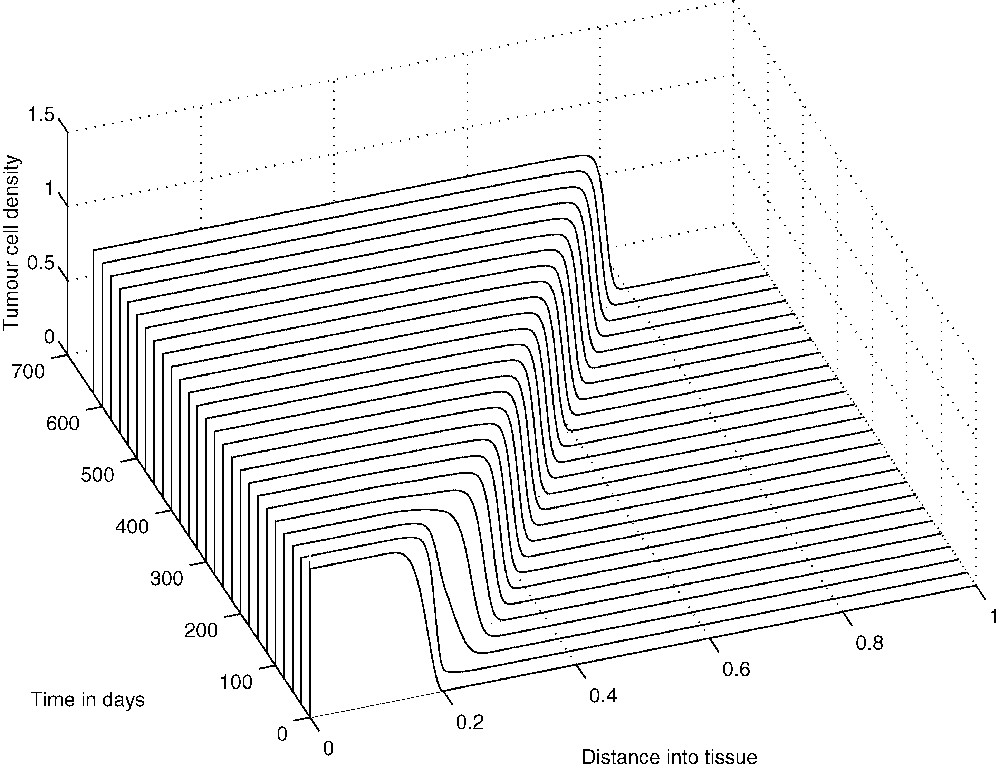
The evolution from the initial conditions of the ‘invasive’ travelling wave of tumour-cell density.

Fig. 14
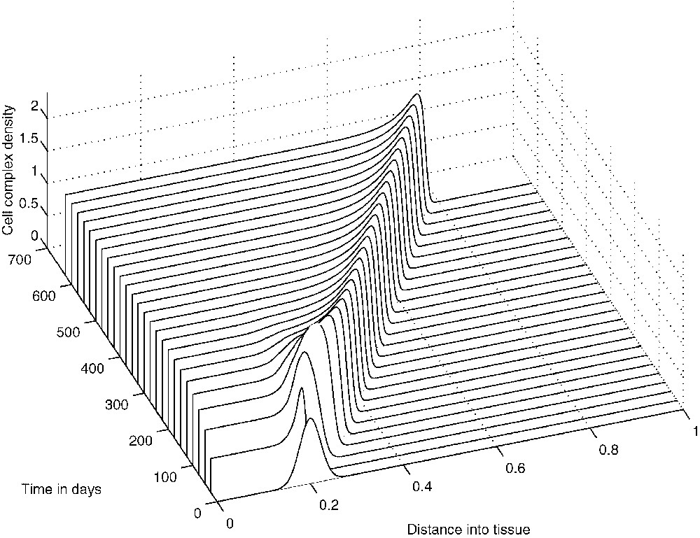
The evolution from the initial conditions of the travelling wave of cell-complex density.

3 Travelling-wave analysis

The numerical simulations of the previous section indicate that the system of Eqs. (9)–(11) exhibits travelling wave solutions for some choice of parameters. Two of the main approaches for establishing travelling-wave solutions for systems of PDEs are: (a) the geometric treatment of an appropriate phase-space, where one essentially is interested in intersections between unstable and stable manifolds and (b) the Leray–Schauder (degree-theoretic) method, which employs homotopy techniques (see e.g. [40,41]). From a numerical analysis point of view, the former approach is used either in conjunction with a shooting method over a truncated domain or by trying to identify a ‘trivial’ heteroclinic connection for some choice of parameters and then follow its deformation as the parameters are changing using numerical continuation.

In all cases the main purpose is to establish the existence of a travelling-wave solution without any available information concerning its nature. Our approach, however, is going to be ‘computer-assisted’ in the sense that we are going to make use of the information that the numerics of the previous section can provide us.

Since we are interested in waves travelling from the left part of the domain to the right, we specify a travelling coordinate $z = x - c t$ , where $c > 0$ and we let:

\tilde{E} (z) = E (x, t), \tilde{T} (z) = T (x, t), \tilde{C} (z) = C (x, t)

We note that we assign the same wave velocity c to each variable, as suggested by the numerical simulations. By substituting

\tilde{E}

,

\tilde{T}

and

\tilde{C}

into the system of Eqs. (9)–(11) and omitting the tildes for the sake of clarity, we get:

- c \frac{d E}{d z} = \frac{d^{2} E}{d z^{2}} + σ + \frac{ρ C}{η + T} - σ E - μ E T + ɛ C

(12)

- c \frac{d T}{d z} = ω \frac{d^{2} T}{d z^{2}} + β_{1} (1 - β_{2} T) T - ϕ E T + λ C

(13)

- c \frac{d C}{d z} = μ E T - ψ C

(14)

Our intention is to take advantage of phase-space techniques and thus we formulate the system of Eqs. (12)–(14) as a dynamical system in

R^{5}

. In particular, by defining the new variables

E_{1} = \frac{d E}{d z} and T_{1} = \frac{d T}{d z}

the system of Eqs. (12)–(14) can be formulated as:

\frac{d x}{d z} = f (x), where x = (\begin{matrix} E_{1} \\ E \\ T_{1} \\ T \\ C \end{matrix}) \in R^{5}

(15)

and

f (x) = (\begin{matrix} - c E_{1} - σ - \frac{ρ C}{η + T} + σ E + μ E T - ɛ C \\ E_{1} \\ - \frac{c}{ω} T_{1} - \frac{β_{1}}{ω} (1 - β_{2} T) T + \frac{ϕ}{ω} E T - \frac{λ}{ω} C \\ T_{1} \\ - \frac{1}{c} μ E T + \frac{1}{c} ψ C \end{matrix})

(16)

Since the wave velocity c is unknown, system (15) can be regarded as a nonlinear eigenvalue problem. Several analytical methods have been developed for estimating c in this framework. However, the numerical solutions of Eqs. (9)–(11) readily yield a value of $c \approx 850$ . In the analysis that follows, we therefore use this numerical estimate for c to fix the wave speed at the constant (non-dimensional) value of 850 and hence take c as a fixed parameter.

The steady states of system (15) can be found by solving the (nonlinear) equation $f (x) = 0$ . Several numerical optimization methods can be employed for this task. However, for the purposes of the travelling-wave analysis, the numerical simulations of the previous section indicate that we should identify a heteroclinic connection between $x^{0}$ and $x^{1}$ , where:

x^{0} \approx (\begin{matrix} 0 \\ 0.62 \\ 0 \\ 0.97 \\ 1.24 \end{matrix}) and x^{1} = (\begin{matrix} 0 \\ 1 \\ 0 \\ 0 \\ 0 \end{matrix})

(17)

One can improve the estimate for

x^{0}

by using the above value as an initial condition in an optimisation algorithm. This would also confirm that

x^{0}

is indeed a steady state of system (15). The fact that

x^{1}

is also a steady state of (15) is trivial.

We are interested in the existence of an orbit $x_{con} (z)$ of (15) that satisfies:

\lim_{z \to - \infty} x_{con} (z) = x^{0} and \lim_{z \to \infty} x_{con} (z) = x^{1}

(18)

We consider the linearizations

\frac{d x}{d z} = D f (x^{0}) x and \frac{d x}{d z} = D f (x^{1}) x

(19)

of the vector field f at equilibria

x^{0}

and

x^{1}

, respectively. It is a straightforward task to determine the spectrum of the Jacobian matrices

D f (x^{0})

and

D f (x^{1})

. Indeed, there are five real eigenvalues of

D f (x^{0})

, three positive and two negative, with the positive ones implying the existence of a three-dimensional unstable manifold

W^{u} (x^{0})

. Furthermore, there are five real eigenvalues of

D f (x^{1})

, two positive and three negative, with the negative ones implying the existence of a three-dimensional stable manifold

W^{s} (x^{1})

. We note that

\dim (W^{u} (x^{0})) + \dim (W^{s} (x^{1})) = \dim R^{5} + 1

(20)

Eq. (20) suggests that

W^{u} (x^{0})

and

W^{s} (x^{1})

probably intersect transversally¹ along an one-dimensional curve in the five-dimensional phase-space [42,43]. If this is the case then this curve would define a (generic) heteroclinic connection.

The values of the parameters of the system under discussion suggest that an approximation of the connecting orbit by perturbing the system of Eqs. (12)–(14) can be feasible. In particular, we perturb Eqs. (12) and (13) by ignoring the effect of the second derivatives on the system (see also [44]). That is to say, we consider the perturbed system:

- c \frac{d E}{d z} = σ + \frac{ρ C}{η + T} - σ E - μ E T + ɛ C

(21)

- c \frac{d T}{d z} = β_{1} (1 - β_{2} T) T - ϕ E T + λ C

(22)

- c \frac{d C}{d z} = μ E T - ψ C

(23)

We note here that by ignoring the second derivatives in effect we choose to focus on a first-order approximation to Eqs. (12) and (13).

Let $Π (x^{0})$ and $Π (x^{1})$ be the projections of $x^{0}$ and $x^{1}$ onto the phase-space defined by Eqs. (21)–(23). It is obvious that $Π (x^{0})$ and $Π (x^{1})$ are steady states of the perturbed system. There is a three-dimensional unstable manifold $W^{u} (Π (x^{0}))$ associated with $Π (x^{0})$ and a one-dimensional stable manifold $W^{s} (Π (x^{1}))$ associated with $Π (x^{1})$ . We have used XPP (see [37]) to investigate numerically the phase-space of the system of Eqs. (21)–(23). XPP provides the implementation of numerical algorithms for tracking one-dimensional invariant manifolds and in the case of $Π (x^{1})$ it was able to confirm that $W^{s} (Π (x^{1}))$ defines a heteroclinic connection between $Π (x^{0})$ and $Π (x^{1})$ . Figs. 15–17 show approximations to the connecting orbit defined by $W^{s} (Π (x^{1}))$ in the $(E, z)$ , $(T, z)$ and $(C, z)$ planes, respectively. These compare very well with the results of the spatio-temporal simulations of the full PDE system.

Fig. 15
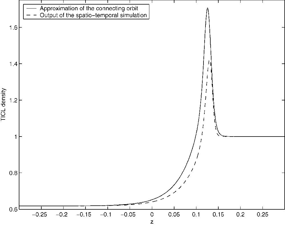
Figure showing the approximation of the connecting orbit in the (E,z)-plane from the travelling-wave analysis (solid line). The orbit was computed over the truncated domain [−0.3,0.3].

Fig. 16
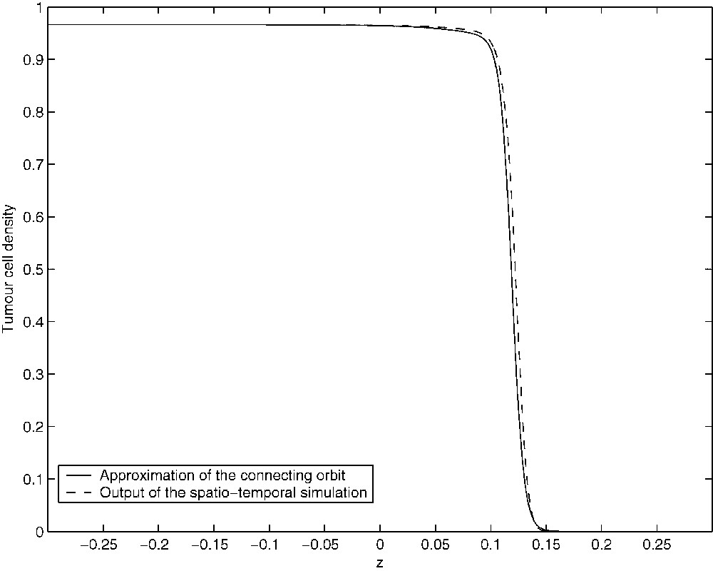
Figure showing the approximation of the connecting orbit in the (T,z)-plane (solid line). The orbit was computed over the truncated domain [−0.3,0.3].

Fig. 17
Figure showing the approximation of the connecting orbit in the (C,z)-plane (solid line). The orbit was computed over the truncated domain [−0.3,0.3].

4 Discussion

In this paper we have undertaken a travelling-wave analysis of a mathematical model developed in [15], describing the growth of solid tumours in the presence of an immune system response. For a particular choice of parameters, the model is able to simulate the phenomenon of cancer dormancy; a clinical condition that has been observed in breast cancers, neuroblastomas, melanomas, osteogenic sarcomas, and in several types of lymphomas. The behaviour of the cancer dormancy simulations can be described as highly irregular, depicting unstable and heterogeneous tumour cell distributions that are nonetheless characterized by a relatively low total number of tumour cells. This behaviour is consistent with several immunomorphological investigations with tumour spheroids infiltrated by TICLs.

However, the alteration of certain parameters of the model is enough to induce bifurcations into the system, which in turn result in the evolution of travelling-wave-like solutions in the numerical simulations. These travelling waves are of great importance because, when they exist, the tumour invades the healthy tissue at its full potential. The existence of these travelling waves for a particular choice of parameters was established in this paper for a reduced system, which nonetheless captures the essential elements of the full model presented in [15].

We would like to note here that the first order approximation employed in deriving Eqs. (21)–(23) could be further investigated in the context of geometric perturbation theory. More precisely, we believe that Fenichel's invariant manifold theorem [42,45] has a special role to play here and, as a matter of fact, it seems that one could try to analyse system (15) by employing the relevant techniques discussed in [42]. Nonetheless, several problems arise in this direction with perhaps the most prominent of them being the unavailability of simple analytic expressions for the steady states of the system under discussion.

The work presented here complements the bifurcation analysis undertaken in [15] and seems to provide an adequate framework for studying and identifying critical parameters of the process in which cancer cells are present in a tissue but do not clinically occur for a long period of time, but can begin to grow progressively at a later date. Thus our modelling and analysis offers the potential for quantitative analysis of mechanisms of tumour-cell–host-cell interactions and for the optimisation of tumour immunotherapy and genetically engineered anti-tumour vaccines.

Acknowledgments

We would like to thank Dr. Fordyce Davidson for the helpful and stimulating discussions. Both authors acknowledge support from the EU Network Grant HPRN-CT-2000-00105 ‘Using mathematical modelling and computer simulation to improve cancer therapy’.

¹ See also the discussion on p. 120 of [43] concerning the so-called transversality theorem.

Bibliographie

[1] V. Schirrmacher T-cell immunity in the induction and maintenance of a tumour dormant state, Semin. Cancer Biol., Volume 11 (2001), pp. 285-295

[2] J.W. Uhr; R. Marches Dormancy in a model of murine B cell lymphoma, Semin. Cancer Biol., Volume 11 (2001), pp. 277-283

[3] E. Yefenof Cancer dormancy: from observation to investigation and onto clinical intervention, Semin. Cancer Biol., Volume 11 (2001), pp. 269-270

[4] A. Alsabti Tumour dormant state, Tumour Res., Volume 13 (1978) no. 1, pp. 1-13

[5] N. Breslow; C.W. Chan; G. Dhom; R.A. Drury; L.M. Franks; B. Gellei; Y.S. Lee; S. Lundberg; B. Sparke; N.H. Sternby; H. Tulinius Latent carcinoma of prostate at autopsy in seven areas, Int. J. Cancer, Volume 20 (1977) no. 5, pp. 680-688

[6] L. Holmberg; M. Baum Work on your theories!, Nat. Med., Volume 2 (1996) no. 8, pp. 844-846

[7] J.A. Aguirre Ghiso Inhibition of FAK signaling activated by urokinase receptor induces dormancy in human carcinoma cells in vivo, Oncogene, Volume 21 (2002) no. 16, pp. 2513-2524

[8] T. Udagawa; A. Fernandez; E.G. Achilles; J. Folkman; R.J. D'Amato Persistence of microscopic human cancers in mice: alterations in the angiogenic balance accompanies loss of tumor dormancy, FASEB J., Volume 16 (2002) no. 11, pp. 1361-1370

[9] P.G. Coulie Human tumor antigens recognized by T cells: new perspectives for anti-cancer vaccines?, Mol. Med. Today, Volume 3 (1997), pp. 261-268

[10] D. Loeffler; S. Ratner In vivo localization of lymphocytes labeled with low concentrations of HOECHST-33342, J. Immunol. Methods, Volume 119 (1989), pp. 95-101

[11] R.A. Deweger; B. Wilbrink; R.M.P. Moberts; D. Mans; R. Oskam; W. den Otten Immune reactivity in SL2 lymphoma-bearing mice compared with SL2-immunized mice, Cancer Immunol. Immunother., Volume 24 (1987), pp. 1191-1192

[12] G. Forni; G. Parmiani; A. Guarini; R. Foa Gene transfer in tumour therapy, Ann. Oncol., Volume 5 (1994), pp. 789-794

[13] E.M. Lord; G. Burkhardt Assessment of in situ host immunity to syngeneic tumours utilizing the multicellular spheroid model, Cell. Immunol., Volume 85 (1984), pp. 340-350

[14] K.M. Wilson; E.M. Lord Specific (EMT6) and non-specific (WEHI-164) cytolytic activity by host cells infiltrating tumour spheroids, Br. J. Cancer, Volume 55 (1987), pp. 141-146

[15] A. Matzavinos; M.A.J. Chaplain; V.A. Kuznetsov Mathematical modelling of the spatio-temporal response of cytotoxic T-lymphocytes to a solid tumour, Math. Med. Biol. IMA, Volume 21 (2004), pp. 1-34

[16] J.A. Sherratt; M.A. Lewis; A.C. Fowler Ecological chaos in the wake of invasion, Proc. Natl Acad. Sci. USA, Volume 92 (1995), pp. 2524-2528

[17] D. Ambrosi; N. Bellomo; L. Preziosi Modelling tumor progression, heterogeneity, and immune competition, J. Theor. Med., Volume 4 (2002), pp. 51-65

[18] L. Arlotti; A. Gamba; M. Lachowicz A kinetic model of tumor/immune system cellular interactions, J. Theor. Med., Volume 4 (2002), pp. 39-50

[19] E. De Angelis; M. Delitala; A. Marasco; A. Romano Bifurcation analysis for a mean field modelling of tumor and immune system competition, Math. Comput. Model., Volume 37 (2003), pp. 1131-1142

[20] N. Bellomo; A. Bellouquid; E. De Angelis The modelling of the immune competition by generalized kinetic (Boltzmann) models: Review and research perspectives, Math. Comput. Model., Volume 37 (2003), pp. 65-86

[21] N. Bellomo; B. Firmani; L. Guerri Bifurcation analysis for a nonlinear system of integro-differential equations modelling tumor-immune cells competition, Appl. Math. Lett., Volume 12 (1999), pp. 39-44

[22] N. Bellomo; L. Preziosi Modelling and mathematical problems related to tumor evolution and its interaction with the immune system, Math. Comput. Model., Volume 32 (2000), pp. 413-452

[23] M.R. Owen; J.A. Sherratt Pattern formation and spatio-temporal irregularity in a model for macrophage-tumour interactions, J. Theor. Biol., Volume 189 (1997), pp. 63-80

[24] M.R. Owen; J.A. Sherratt Modelling the macrophage invasion of tumours: Effects on growth and composition, IMA J. Math. Appl. Med. Biol., Volume 15 (1998), pp. 165-185

[25] M.R. Owen; J.A. Sherratt Mathematical modelling of macrophage dynamics in tumours, Math. Models Methods Appl. Sci., Volume 9 (1999), pp. 513-539

[26] J.A. Sherratt; A.J. Perumpanani; M.R. Owen Pattern formation in cancer (M.A.J. Chaplain; G.D. Singh; J.C. McLachlan, eds.), On Growth and Form: Spatio-Temporal Pattern Formation in Biology, John Wiley & Sons Ltd, 1999

[27] S.D. Webb; J.A. Sherratt; R.G. Fish Cells behaving badly: a theoretical model for the Fas/FasL system in tumour immunology, Math. Biosci., Volume 179 (2002), pp. 113-129

[28] C.E. Kelly; R.D. Leek; H.M. Byrne; S.M. Cox; A.L. Harris; C.E. Lewis Modelling macrophage infiltration into avascular tumours, J. Theor. Med., Volume 4 (2002), pp. 21-38

[29] V.A. Kuznetsov; G.D. Knott Modeling tumor regrowth and immunotherapy, Math. Comput. Model., Volume 33 (2001), pp. 1275-1287

[30] V.A. Kuznetsov; I.A. Makalkin; M.A. Taylor; A.S. Perelson Nonlinear dynamics of immunogenic tumours: Parameter estimation and global bifurcation analysis, Bull. Math. Biol., Volume 56 (1994), pp. 295-321

[31] U. Foryś Marchuk's model of immune system dynamics with application to tumour growth, J. Theor. Med., Volume 4 (2002), pp. 85-93

[32] Z. Szymańska Analysis of immunotherapy models in the context of cancer dynamics, Appl. Math. Comput. Sci., Volume 13 (2003), pp. 407-418

[33] C.G. Ioannides; T.L. Whiteside T-cell recognition of human tumours – implications for molecular immunotherapy of cancer, Clin. Immunol. Immunopathol., Volume 66 (1993), pp. 91-106

[34] J. Jaaskelainen; A. Maenpaa; M. Patarroyo; C.G. Gahmberg; K. Somersalo; J. Tarkkanen; M. Kallio; T. Timonen Migration of recombinant IL-2-activated T-cells and natural killer cells in the intercellular space of human H-2 glioma spheroids in vitro – a study on adhesion molecules involved, J. Immunol., Volume 149 (1992), pp. 260-268

[35] Y. Kawakami; M.I. Nishimura; N.P. Restifo; S.L. Topalian; B.H. O'Neil; J. Shilyansky; J.R. Yannelli; S.A. Rosenberg T-cell recognition of human-melanoma antigens, J. Immunother., Volume 14 (1993), pp. 88-93

[36] H. Siu; E.S. Vitetta; R.D. May; J.W. Uhr Tumour dormancy, regression of BCL tumour and induction of a dormant tumour state in mice chimeric at the major histocompatibility complex, J. Immunol., Volume 137 (1986), pp. 1376-1382

[37] G.B. Ermentrout Simulating, Analyzing, and Animating Dynamical Systems: A Guide to XPPAUT for Researchers and Students, Software, Environments, and Tools, vol. 14, SIAM, 2002

[38] A. Dhooge; W. Govaerts; Yu.A. Kuznetsov MATCONT: A MATLAB package for numerical bifurcation analysis of ODEs, ACM Trans. Math. Software, Volume 29 (2003), pp. 141-164

[39] A. Dhooge; W. Govaerts; Yu.A. Kuznetsov Numerical continuation of fold bifurcations of limit cycles in MATCONT, Lect. Notes Comput. Sci., Volume 2657 (2003), pp. 701-710

[40] H. Berestycki; B. Larrouturou; P.L. Lions Multi-dimensional travelling wave solutions of a flame propagation model, Arch. Rational Mech. Anal., Volume 111 (1990), pp. 33-49

[41] A.I. Volpert; V.A. Volpert; V.A. Volpert Traveling Wave Solutions of Parabolic Systems, Translations of Mathematical Monographs, vol. 140, American Mathematical Society, 2000

[42] P.B. Ashwin; M.V. Bartuccelli; T.J. Bridges; S.A. Gourley Travelling fronts for the KPP equation with spatio-temporal delay, Z. Angew. Math. Phys., Volume 53 (2002), pp. 103-122

[43] J. Guckenheimer; P. Holmes Nonlinear Oscillations, Dynamical Systems, and Bifurcations of Vector Fields, Applied Mathematical Sciences, vol. 42, Springer, 1983 (corrected seventh printing, 2002)

[44] S.R. Dunbar Travelling wave solutions of diffusive Lotka–Volterra equations, J. Math. Biol., Volume 17 (1983), pp. 11-32

[45] N. Fenichel Geometric singular perturbation theory for ordinary differential equations, J. Differ. Equat., Volume 31 (1979), pp. 53-98

Commentaires - Politique