

1 Introduction
The purpose of this paper is to analyse, from a numerical point of view, some aspects in the evolution of a population of Gambussia affinis or mosquitofish as an example of a size-structured population model. We show how to study the dynamics of a model from numerical techniques. First, it is appropriate to use different numerical integrators and compare the corresponding results. Such comparisons allow us to achieve some certainty regarding different questions in the dynamics of the population. From this, we can choose the numerical method which shows the best adaptation to the problem. With the help of the most efficient scheme we study the evolution of the population in order to evaluate the values and deficiencies of the model proposed. One of the relevant properties discovered is that, with appropriate vital functions, the population tends to be periodic and stable.
One of the ways to study the dynamics of species in biology or ecology is based on the so-called structured models. In these models, one or more internal variables of the individuals, like age, size, etc., allow us to show the effect of the physiological state of the individuals on the population dynamics. At the same time, these models incorporate vital functions like mortality, fertility, etc., generally in nonlinear form (with nonlocal terms). The way these vital functions depend on the structural variables and density of population determines the adaptation of the model to the real behaviour of the species [1–4].
In many cases, size is the individual parameter which has more influence on the evolution of the population. The ability of individuals to survive and reproduce depends on it. This gave rise to the consideration of the so-called size-structured mathematical models. The first models of this type were proposed in [5,6] and generalized the well-known age-structured models [7,8]. A general size-structured population model can be described by the following equations:
| (1.1) |
| (1.2) |
| (1.3) |
| (1.4) |
The so-called vital functions of the population, which determine the life history of an individual, are given by the functions g, α and μ, representing, respectively, growth, fertility and mortality rates. All the functions in the model are nonnegative and depend on size and time. This time dependence implies a possible seasonal behaviour of the population. Finally, in order to consider the influence of individuals with different size on life conditions, the vital functions can also depend on the total number of individuals. This is indicated by the integrals (1.4), , and , which average the density of the population by using specified functions , and .
Eq. (1.1) is a PDE with nonlocal terms representing the balance law of the population. It describes the evolution of the number of individuals with a given size due to growth and mortality. Eq. (1.2) is a nonlocal boundary condition which represents the birth law of the population. Finally, the initial distribution of the density is given by Eq. (1.3).
It is also usually assumed that
| (1.5) |
The paper is structured as follows. In Section 2, we study the evolution of a population of mosquitofish, from the general equations (1.1)–(1.4). We introduce significative hypotheses in the model, the equations and the selection of the vital functions with their biological properties. The type of these functions and the initial condition is determined both from a biological and mathematical point of view. In the latter case, one of the most noticeable properties is regularity. Smooth functions are initially chosen for numerical reasons of convergence of the methods used. This selection is different from the one considered in Ref. [10] and has a relevant influence on the numerical results and also in a biological sense. Section 3 is a numerical study of the model. In general, the analytical resolution of models like (1.1)–(1.4) is not possible; thus it is necessary to use numerical integration to obtain information about the behaviour of the population under consideration. This study is based on two questions. First, we analyse the efficiency of four numerical methods for solving the problem. This allows us to choose the schemes which, in our opinion, are the most appropriate for the model considered. Also, with the methods selected, we introduce a numerical analysis of the model for long times. This previous numerical study leads us to consider a final biological discussion of the model. Here, we first describe the behaviour of the population in one year. Finally, the analysis for long times shows new topics such as the periodicity in the evolution of the population. This tendency to periodicity seems to be a property of the model since it occurs for different initial conditions. Some other phenomena, such as overcrowding or extinction, may take place if the mortality rate, which includes the only nonlinearity in the model, is changed.
2 Gambussia affinis model
The biological model which our study focuses on analyses the dynamics of a population of the so-called Gambussia affinis or mosquitofish. Sulsky [10] analyses some numerical questions in the integration of a model similar to (1.1)–(1.4) by building vital functions from experimental data, including seasonal hypotheses. Functions used by Sulsky are, in general, -piecewise, with an initial condition and a mortality rate represented by discontinuous functions.
Sulsky introduced some hypotheses in the model in order to simplify the study. First, length is used in the model as the variable which represents individual size. This quantity is measured in milimetres, within a range between and . She also chose the day as a unit of measure for temporal evolution. Furthermore, she assumed that the model uses the same size distribution for males and females. Therefore, only the population of females is considered and denotes the density of females with length x at time t. Finally, she only considered the influence of the number of individuals of different size in the mortality. This dependence is represented by the function
| (2.1) |
| (2.2) |
| (2.3) |
| (2.4) |
The use of (2.1)–(2.4) to describe the dynamics of a population of Gambussia affinis requires the specification of the vital functions, fertility , growth and mortality rates. Our proposal, based on the study of Sulsky [10], assumes, as she does, dependence of the vital functions with respect to seasons, with a periodic character. The most important difference in our study is the use of smoother data, functions with more regularity. This selection is motivated by two reasons. The first is of a numerical character: the numerical methods we use are of order two, hence it is theoretically necessary some regularity of data in order to make them work. We have carried out experiments with less regular data and the results do not change significatively although efficiency is lost. On the other hand, we think that the use of smoother functions is more realistic from a biological point of view and establishes new proposals in the model. Therefore, we have constructed -functions which are periodic in time (with annual periodicity) and that satisfy the compatibility conditions so that the solution to the problem is of a -type.
Now, we describe in detail our selection of the vital functions. We first consider the fertility rate which we suppose in the form . Here, we have used field data by Krumholtz [11], which relates the length of gravid females to the number of young they have. In order to fit Krumholtz's data, , we choose the function as a smooth spline which minimizes the functional
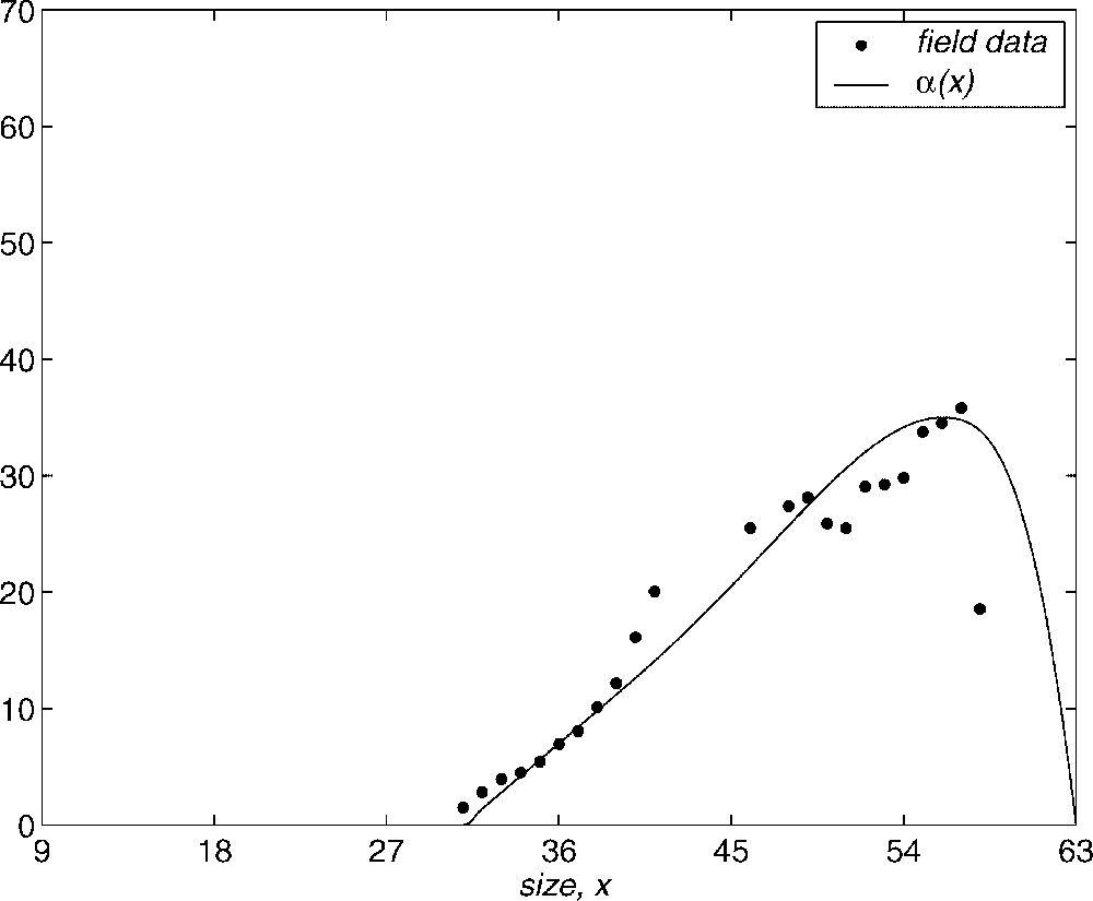
Shape of α(x) function.
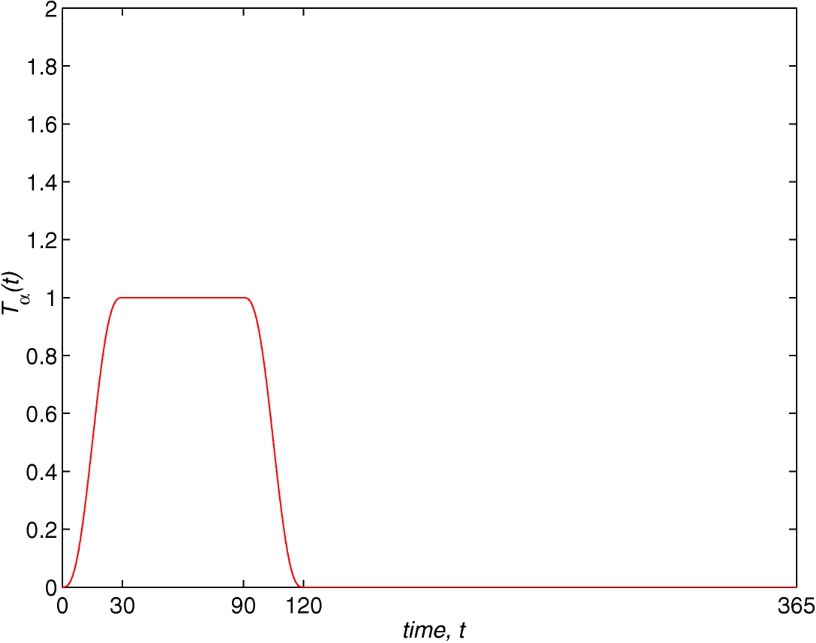
On the other hand, it is necessary to include dependence on time, because fertility is affected by seasons. We choose the function as
This function is periodic with period days and includes the fact that during a year there is only a season of 120 days when the population is fertile. The breeding season begins in May (see Krumholtz data [11]). The birth rate increases regularly as a quintic polynomial during the first month until it reaches a maximum value for the next two months. Then it decreases to zero during the following month while no births occur during the rest of the year. The same behaviour takes place every year.
The growth rate is also assumed in the form . The function g is
This belongs to the type of growth curves proposed by von Bertalanffy [12] and takes into account that a newborn with a length of 9 mm takes about six weeks to reach an adult length of 31 mm. Furthermore, the function g is zero for the maximum length allowed (63 mm) and it is of the type which makes that (1.5) holds.
The growth also varies with the season. The function is also -periodic with
Now, we describe the mortality rate, which includes the nonlinearity of the model. Bostford et al. [13] estimate the instantaneous per capita mortality rate for females with a length larger than 30 mm. They consider the quantity
Our proposal assumes a mortality rate of the form , . The function is a regularization of the discontinuous function considered by Sulsky [10]
| (2.5) |
Mortality also varies seasonally. The function is
The mortality function depends on the number of individuals by means of the quantity described in (2.1). The weight function represents the way total population affects the mortality of the youngest. In our case, this dependence is exclusively due to the immature fish, showing the behaviour of juveniles with respect to predation and competition for limited resources. Explicitly,
3 Numerical approximation
As it was observed in Section 1, the analytical resolution of the Gambussia problem is not possible. Thus our study has to be carried out by using numerical integration and includes information of two types: the first one is quantitative. We can obtain results about the density of the population in a fixed time in terms of the size under certain vital conditions. The results can also be of a qualitative type, showing, for instance, a certain behaviour for long times.
This section has two parts. The first one establishes a competition between four numerical schemes, in terms of efficiency and adaptation to the biological problem. This allows us to select the integrator which in our opinion is the most appropriate for the case considered. Secondly, with this method, we discuss the results in a biological sense, describing the relevant properties of the model proposed.
The selection of the numerical method to be used for the experiments is a question to take into account. It is natural to consider those methods that, giving a good approximation to the solution to problems like (2.1)–(2.4), their computational efficiency is appropriate. Therefore, before obtaining conclusions about the population under study through numerical analysis, it is necessary to make a selection between possible numerical integrators, in terms of the various types of efficiency. Then, the analysis of the model from numerical techniques requires two stages: first, we have to consider different numerical integrators and reject those which give results with no biological sense or with little computational efficiency. A second stage consists of obtaining conclusions about the dynamics of the model, studying its values and deficiencies by using the best of the numerical methods employed. In the literature, we can find some studies in this way for different species, such as the monogonont rotifera whose sexual phase dynamics was studied in [14,15].
Numerical integration of size-structured models is still at a primary stage, especially in the analysis of the convergence of numerical schemes. Roughly speaking, there are basically two classes of numerical schemes for the integration of size-structured problems: the standard finite difference methods (Upwind, Lax–Wendroff, Box) [16] and those schemes based on integration along characteristic curves, where the PDE is transformed into a system of ODE, infinite dimensional, using the characteristic curves. Higher order methods are appropriate for obtaining the solution faster than the others. However, the regularity of the data in real problems is not as high as needed. So, second order schemes maintain a good compromise between the required smoothness and the efficiency of the schemes. The first study was written by de Roos [17], who introduced the escalator boxcar train, a semidiscrete scheme for integrals (momenta) of the density function. Ito et al. [18] introduced a method for the linear problem based on the integration along the characteristic curves by using an invariant grid called natural grid. They proved convergence of second order for initial conditions of compact support. Schemes based on the natural grid have been proposed by different authors, for the linear problem [19,20] and the nonlinear problem [21]. In [22], the approximation to the nonautonomous problem with a growth function depending on size has been analysed by using a second order scheme based on the box method. The analysis of the fully nonlinear problem was initiated by Ackleh et al. [23]. They introduced an implicit finite difference scheme of first order. The first methods of second-order were proposed by Angulo et al. [24]. These methods are based on the integration along the characteristic curves, with a dynamic construction of the grid to improve the efficiency. On the other hand, the diversity of the numerical methods used for the problem also generates works about efficiency [10,22]. One conclusion which can be deduced from them is that methods that integrate along the characteristic curves are probably more efficient. However, as it is revealed in [22], the choice of the numerical method probably depends on the particular problem to be solved. Finally, we can find an extensive revision in [26], focused on the physiologically-structured models, which extends the study made in [26] for the age-structured ones.
3.1 Numerical results
In our case, we have considered two difference methods of second order, the Lax–Wendroff scheme [10,22] and box method [22] and two characteristics methods, Aggregation Grid Nodes method (AGN) and Selection Grid Nodes method (SGN) [24] to study the problem (2.1)–(2.4). All the schemes are briefly described in Appendix A. The Lax–Wendroff method is an explicit scheme with an easy implementation on a uniform grid. The box method is an implicit scheme on a uniform grid. Therefore, a nonlinear system of equations at each time step has to be solved by means of an iterative technique [22]. Both AGN and SGN methods are explicit and implemented in a nonuniform spatial grid. In the case of the AGN scheme, the number of grid nodes grows at each time step, making the computational cost in the long-time numerical integration more expensive. The SGN method avoids this cost by means of a selection strategy applied to each time step. They are described and analysed in [24].
We assume an initial distribution of the form
| (3.1) |
Note that the initial population only contains adults. This fact is congruent with the hypothesis that the initial time corresponds to the beginning of the fertile period of the population. It is also supposed that, if an individual which was born on the last day of the fertile period of the last year has survived, then its length is greater than 31 mm.
3.1.1 Efficiency study
First, we show some experiments in order to determine the adaptation of the methods to the problem. In Fig. 2 the evolution in a year of the total population
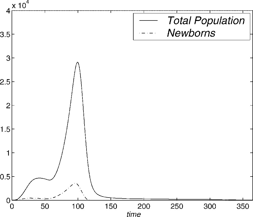
Evolution of total population and newborns with time (days).
For a final time of one year we present, for each method, a figure which shows the value of the numerical solution as a function of the length at time .
We begin with the results obtained by the Lax–Wendroff scheme. We should point out that this method must satisfy the Courant–Friedrichs–Levy (CFL) condition. A more complete discussion of this method can be found in general studies on the numerical solution to partial differential equations like, for example, the work of Morton and Mayers [16]. To the best of our knowledge, the convergence of such a scheme for the solution to size-structured population models has still to be carried out. Numerical experiments in the literature [22] suggest that the method is of second order. The most efficient results correspond to the values of , closer to the one determined by the CFL condition (in this case ). Taking in Fig. 3, we show the numerical solution with , ( and ) and a computational cost of 8.49 CPU-time (the CPU-time will be always measured in seconds). We note that some spurious oscillations appear, giving, in some cases, a negative population that has no biological meaning and that could damage the long time integration. This behaviour is not acceptable for greater values of k and h, although these oscillations tend to disappear as the discretization parameters are smaller. The results are even worse for smaller values of r, as we have confirmed with different experiments.
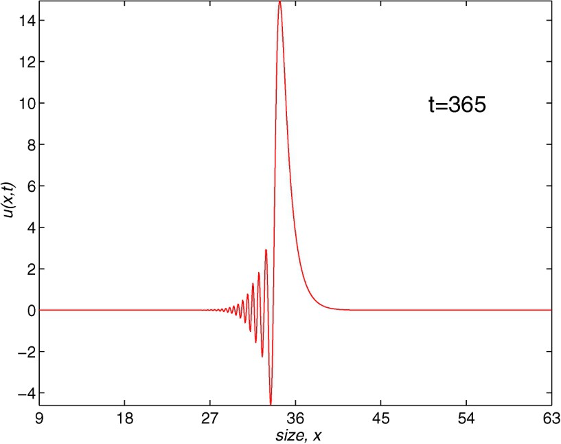
Population density with length. The Lax–Wendroff method, t=365, J=864, N=5840.
Next, we deal with the behaviour of the box method. In the form given in [22], the scheme is truly implicit and at each time step the nonlinear equations must be solved by some fixed-point iteration procedure. Again, the text of Morton and Mayers can be useful in finding more properties of this scheme and we should point out that the authors emphasize the difficulty of carrying out convergence analysis even in the simple cases [16, p. 110]. However, the numerical method is second-order accurate as h tends to zero assuming that the time step is of the form , with r an arbitrary and positive constant fixed throughout the analysis. The stability and convergence analysis in the cases of an age-structured and a nonautonomous size-structured population model has been derived [25,26]. We should also point out that, contrary to the rest of the methods employed in this section, the box scheme does not make use of (1.5) in the case of size-structured population models. Therefore, this method can be used with more general models where this condition does not appear. Our experience with the box method leads us to use parameter values with a relation greater than the one considered for the Lax–Wendroff scheme. In Fig. 4, we show the numerical solution obtained with , (, ) corresponding to and a computational cost of 1.63 CPU-time. Here, we observe some oscillations in the final profile. This could provide wrong information about the solution. When using , we need more CPU-time in order to make these oscillations disappear, since an appropriate number of nodes in the spatial grid is necessary. On the other hand, in our experiments with , we need more CPU-time to obtain good profiles; in this case some oscillations, similar to those of the Lax–Wendroff method with less computational cost, appear.
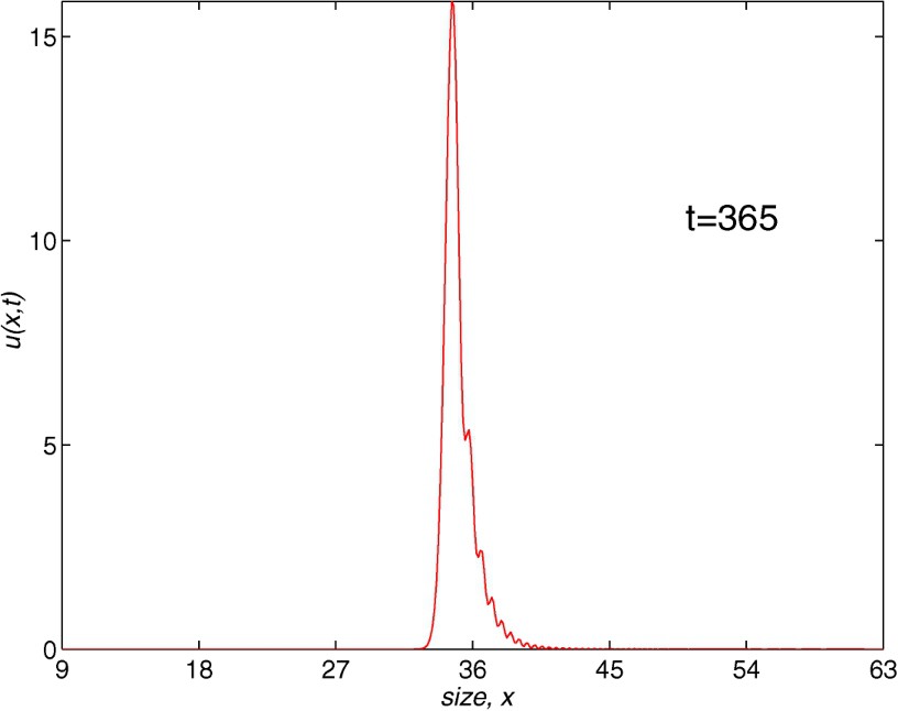
Population density with length. The box method, t=365, J=432, N=730.
Next, we have considered the numerical integration of the problem with the characteristics schemes introduced in [24]. We should note that, in the case of AGN method, the number of nodes grows at each time level because a new node is introduced at each time step. The SGN-scheme avoids the increasing number of nodes by using a selection of them at each time level. These two methods are the first two second-order schemes which solve the fully nonlinear model. The convergence of the schemes was carried out in [24]. In Fig. 5, we show the results obtained with both methods. We have used , (, ) with , which implies a CPU-time of 1.24 for the first method and , (, ) with and 0.20 CPU-time for the second one. The values of r are presented as the most efficient in the exhaustive experimentation with different parameters. The profiles obtained in both cases are smooth and no oscillations appear. Besides, the computational cost is much smaller than the one needed for the finite difference methods. Therefore, Aggregation and Selection Grid Nodes methods are the most appropriate for the biological example, while the Lax–Wendroff scheme is the worst, since it needs much more CPU-time to obtain a profile of the solution without oscillations.
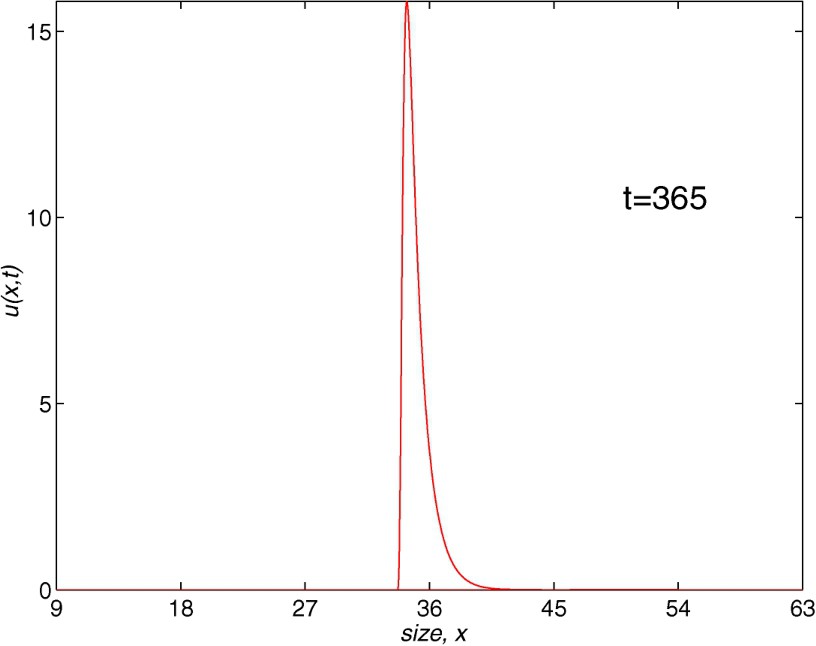
Population density with length. AGN (J=54, N=1460) and SGN methods (J=216, N=730), t=365.
From a more quantitative point of view, the results are very similar. In Fig. 6, we present, in a logarithmic scale, an efficiency plot where we show the error as a function of the computational time (in seconds). In the case of the computation of the error, since we do not know the exact solution to this problem, we obtain a numerical approximation to the total population at time with small enough discretization parameters, for each numerical scheme. These values are very closed among them and we can consider them as the theoretical one. Thus, for another values of the parameters h and k the corresponding error is obtained by comparing the approximation to the total population with the considered as the theoretical one. Next, we build, for each numerical scheme, a tableau with the errors corresponding to different values of the parameters k and h. Now, by means of the procedure employed in [22], we discovered the most efficient value of r (for each method) and, finally, we compare all the schemes in Fig. 6. These values of r have been introduced previously.
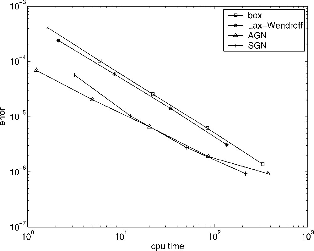
Error vs. CPU-time. Lax–Wendroff method (∗), box method (□), AGN scheme (▵), SGN method (+).
Fig. 6 shows that the most efficient methods are the characteristics schemes, and the best one corresponds to the SGN method. The behaviour of the AGN method is better as less computational time is employed. It begins to be less efficient when the number of nodes grows with the corresponding computational cost increment. In this last case, the difference methods are close to the efficiency of the AGN scheme. Among the difference methods, the Lax–Wendroff scheme is more efficient than the box method. (We recall that this method is implicit.) However, the distance between them is not as large as we previously could suppose, because the box method provides more freedom to choose the parameter values (k and h) than the Lax–Wendroff scheme, since this scheme must satisfy the CFL condition.
Finally, we should note that our study is made with -piecewise data functions and with compatible initial and boundary data. If we were unable to reach such smoothness or the initial and boundary data were not compatible, the behaviour of the difference methods would be even worse, except for the box with . On the other hand, the characteristics methods dynamics is good enough and they are shown to be as the most efficient schemes [15,25].
3.1.2 Long-time behaviour
We now study the evolution of the population of mosquitofish. The numerical integration for long times requires to control the spurious oscillations, in order to avoid inappropriate results. Thus we have analysed the integration of the biological example for a period of ten years by using the methods which integrate along the characteristic curves. As we have seen previously, they achieve a smooth solution profile in a more efficient way.
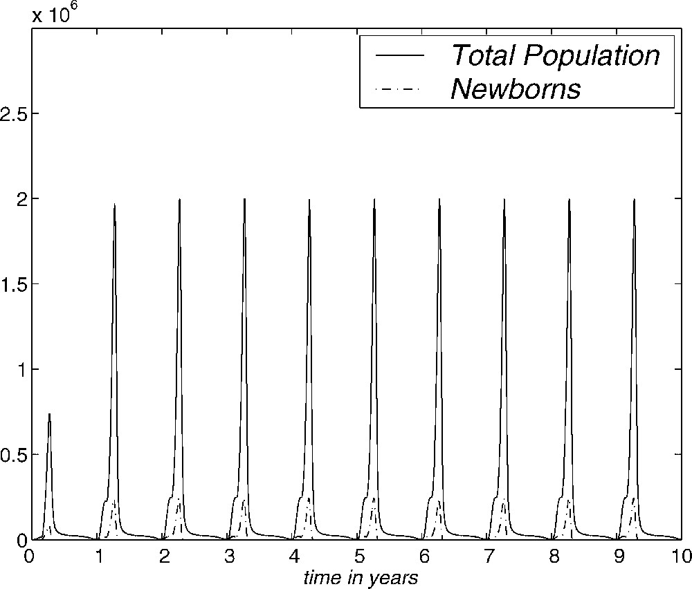
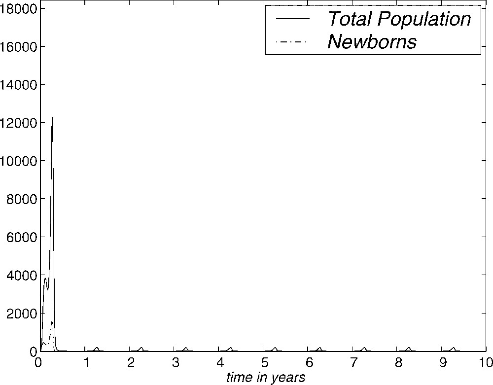
In Fig. 7, we show the evolution over ten years of the numerical approximation to the total population and the number of newborns obtained with the AGN and SGN methods. Here we have used , , with a CPU-time of 12.4 in the case of the AGN method and , and a CPU-time of 0.5 for the SGN method. This figure shows that the behaviour of mosquitofish population, with an initial distribution given by (3.1), tends to be periodic. This periodic evolution represents the influence of the seasons on the model and we have obtained this behaviour with different initial conditions, even with the one considered by Sulsky [10]. In fact, we have repeated the same experiment with the vital functions selected in [10] and the periodic behaviour has also been obtained, but with greater computational effort. This is one of the reasons why the regularity of vital functions is important.
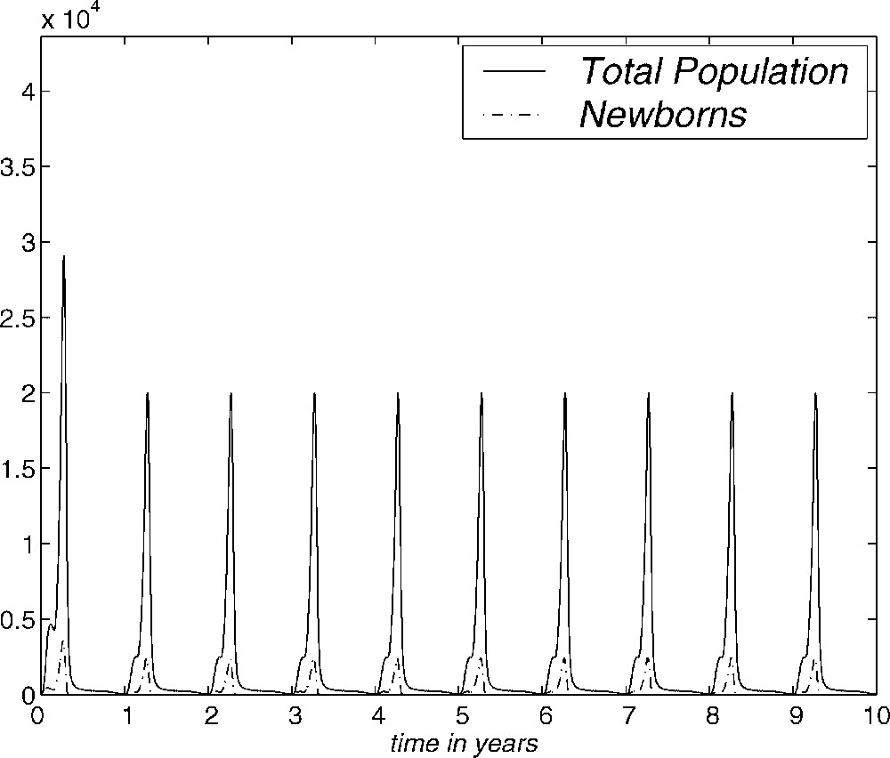
Evolution of total population and newborns for ten years. AGN and SGN methods.
Therefore, the periodic evolution of the numerical approximation seems to be a property of the model. The SGN method is, in this case, more efficient than the AGN method, since the first one achieves the periodic behaviour of the total population and the number of newborns with much less computational time.
The study made in the previous subsection, which includes an appropriate selection of the parameters k and h (that is, the parameter r), is necessary. If we employ the Lax–Wendroff method, the box scheme or the AGN and SGN methods with smaller values of r than those employed here, the solution to the problem could not be obtained for long values of T.
3.2 Biological discussion of the model
In this subsection, we study the model from a biological point of view. First we explain the vital functions involved in the problem and then we describe some biological conclusions from the numerical results.
The model employed for the solution to the Gambussia problem is structured: this means that the dynamics of the population are determined by the vital functions defined in Section 2. The fertility rate is considered as . Function is built using the field data (see Fig. 1), where we assume that the fertile females have a size longer than 31 mm and the fertility increases with the size. The maximum is reached at 54 mm and then it declines to zero at the maximum size. In order to take into account the seasonal behaviour, this is multiplied by a periodic function (with a period equal to 365 days) so that the fertile period are the months between May and August and the maximum fertility is reached in June and July (see Fig. 8). The growth rate is taken as (see Fig. 9) where is chosen as a von Bertalanffy growth curve, which is a classical approach in ecology, and the parameters are obtained by the field data. The function weights the growth in order to show that this is greater at the period of the year with more environmental facilities (June/July) and it maintains a minimum during the months between September and April (both inclusive) while May and August are considered transition months between the extreme situations. Finally, the mortality function is taken in the form of (see Fig. 10). Its behaviour is also seasonal and it is supposed that the maximum mortality period spans the months between September and April and the minimum one corresponds to the months of June and July. According to the studies of Bostford [13], the mortality rate is constant for adults and the choice for the immature fish depends on the total immature population. This last property implies a life of competition among these individuals and demonstrates the influence of the dynamics of the population in the life conditions of immature fish. The mathematical expression of this fact is arbitrary but we will show numerically the existence of a periodic state which is asymptotically stable. This dynamics is coherent with the biological setting. We will also discuss later the role of the constant C in the population dynamics.
Shape of function.
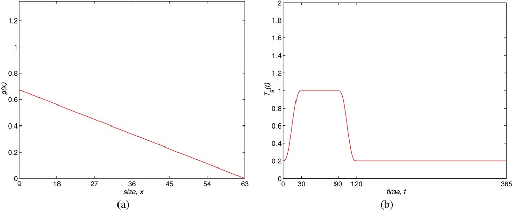
(a) Shape of g(x) function. (b) Shape of function.
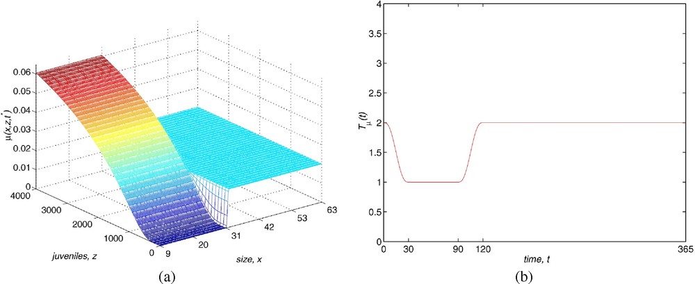
(a) Shape of μ(x,z) function. (b) Shape of function.
Another property of the vital functions is that the individuals do not reach the maximum value in finite time. Moreover, it is easy to show that the flux gu at the maximum size is null.
The previous discussion between the four numerical methods was necessary to establish the most appropriate one to deduce conclusions about the model. The numerical study in Section 3.1 shows that for this problem the most efficient scheme is the SGN method. Therefore, with this integrator, here we will make some remarks, in biological terms, about the model considered in this paper.
For a final time of a year we present some figures which show the value of the numerical solution as a function of the length, at times , , , (end of the fertile period), , and . We first analyse the results from Fig. 11. The choice made of the vital functions implies that at the end of the first month (May, ), the greatest part of the population is immature (4053 immatures and 18 adults) and also the population is clearly divided between juveniles and adults. In the second month , there is a fertile population which has been born in this season. This fact is maintained in the next two months ( and ), a situation which generates the greatest number of births in the season and the fact that the biggest part of the mature population is born in this season. At the end of the fertile period we can show that the mature population of the previous season remains and it starts to diminish until it completely disappears over longer times. Also, in this period (, ), we can show that the profile of the population, which could be considered as an archetype, begins to appear. We can say that the population at the end of the year is only composed of adults. (See Fig. 5.) Also, after the study of the monthly evolution of the newborns, we can affirm that these adults correspond to the live newborns of the last fertile month. The newborns in such a period do not reproduce in the year and they are the only ones with this property. Finally, the third fertile month is the most prolific.
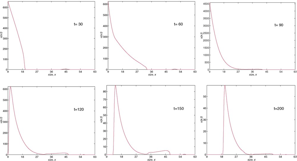
Evolution of population density with length. SGN method, J=216, N=730.
As has been pointed out before, the influence of the seasons is remarkable in Fig. 7. This shows that the total population and newborns tend to be periodic. This behaviour has been obtained with different initial conditions. Therefore, the existence of a periodic solution which is asymptotically stable is shown numerically. This means that the population stabilizes in a state with annual periodicity under the hypotheses considered and by using field data. This annual periodicity is a consequence of the dependence of the vital functions with respect to the seasons. The asymptotic state is determined by the life conditions imposed on the population. They have been deduced from real data where possible. Therefore, under simple hypotheses, and if there is no change in the vital conditions of the population, we have observed that the population reaches a state which allows a specific population with a specific size distribution to survive.
An open question concerns the capacity of the model to reproduce other behaviour of the population. This can depend on the vital functions selected. As an example, we focus on the mortality function. The variation in the parameter of the mortality rate in (2.5) can be interpreted as a change in the life conditions. This is observed in the model by the fact that the asymptotic state allows a larger or smaller number of individuals to survive.
We have already commented that if the constant C in (2.5) is bigger, maximum mortality is reached for greater size, which makes life conditions easier, with less competition and a greater number of resources for the immature population. This should imply growth in the population. In Fig. 12, we show the evolution of the population over ten years by using the SGN method, with a mortality rate of the form (2.5), where . The behaviour of the population again tends to be periodic. However, if we compare this with Fig. 7, we observe that the population grows in two orders of magnitude. This percentage shows a linear dependence of the population, with respect to the value of the constant C, on the mortality function (2.5).
Evolution of total population and the newborns over ten years. SGN method. C=200,000.
Similarly, when the constant C is smaller, life conditions are harder. In Fig. 13, we show the evolution of the population of Gambussia affinis over ten years by using the SGN method with a mortality rate of the form (2.5), where . We observe that when life conditions become harder, the total population of the asymptotic equilibrium does not manage to reach individual. This can be interpreted as the extinction of the population. However, the way this fact is shown mathematically, that is from a periodic function (which therefore does not go to zero) is a deficiency of the model. We will try to improve this in a future work.
Evolution of total population and the newborns over ten years. SGN method. C=20.
Acknowledgments
The authors are very grateful to the referees for their suggestions to improve the paper.
This work has been supported by project BFM2002-01250 and project VA063/04 (Consejería de Educación y Cultura de la Junta de Castilla y León).
Appendix A Numerical methods
A.1 The Lax–Wendroff method [10]
Let J be a positive integer. Let the points of the grid in the size variable be , , where is the grid diameter. We denote by k the time step, and the discrete time levels as , , . The sub-index j makes reference to the grid point and the super-index n to the time level . Finally, we denote by the numerical approximation to , , . We also consider that an approximation to the initial condition (1.3), , is given.
The Lax–Wendroff method is a two-stage scheme defined for each . First we calculate the intermediate values
| (A.1) |
A.2 The Box method [22]
The parameters J, N, h and k are defined as in Appendix A.1.
We introduce the half integer grid points , ; the mean value operators , , and the difference operator .
The box method is defined by
| (A.2) |
| (A.3) |
A.3 Aggregation Grid Nodes method (AGN) [24]
The parameters J, N, h and k are defined as in Appendix A.1.
The initial grid nodes are , . We suppose that the approximations to the theoretical solution in such nodes are known, , . We also suppose that at the first time level , the grid nodes, , and the corresponding solution values, , are known. Furthermore, and , , are (numerically) in the same characteristic curve. Angulo and López-Marcos obtained the initial conditions by means of the well-known second-order method [24].
The numerical approximations at the time level , are obtained as follows. We suppose that the numerical approximations at the previous time levels, and , are known, , and , . Where and , belong (numerically) to the same characteristic curve. We introduce the notation
Also, where , , are the coefficients of the composite quadrature rules of at least second order. This notation will be used throughout the subsection. First, the grid values at the time level are calculated by
| (A.4) |
| (A.5) |
| (A.6) |
| (A.7) |
| (A.8) |
| (A.9) |
| (A.10) |
A.4 Selection Grid Nodes method (SGN) [24]
The following scheme considers a modification in the grid of the previous one so that, by using a selection of the grid nodes, the number of nodes does not increase at each time level. Thus, we try to reduce the computational cost without loss of accuracy.
The grid nodes and the numerical approximations at time , , , are defined by means of (A.4)–(A.10) for . Next, we calculate .
At consecutive time levels, there are different numbers of nodes because a new node that fluxes through the boundary is introduced. So, at the time level , we have grid nodes, at we have and at we have . Now, the first grid node that satisfies
Now, we suppose that the numerical approximations at time levels and are known, and they are denoted by , , and , , (note that and , , are, numerically, in the same characteristic curve). In addition, the grid considered at has lost two nodes with respect to the moment when was actually calculated, while the grid used at has only one node less than . The numerical grid nodes at the new time level , are computed by means of (A.5) and (A.6), , and the approximations to the theoretical solution in these nodes are obtained using (A.7) and (A.8), . The equations at time level are completed with the approximation to using (A.10).
Now, we calculate . Note that, for the time levels , , the quadrature rules always use the same number of nodes . Finally, we eliminate the first grid node that satisfies