Adaptive properties of living beings: Proposal for a generic mechanism. (Self-Programming Machines III)

Jean-Paul Moulin

doi:10.1016/j.crvi.2005.12.002

Biological modelling / Biomodélisation

Adaptive properties of living beings: Proposal for a generic mechanism. (Self-Programming Machines III)

Presented by: Michel Thellier

Jean-Paul Moulin ¹

¹ Département d'information et de recherche médicale, Centre hospitalier interdépartemental de Clermont-de-l'Oise, 2, rue des Finets, 60607 Clermont-de-l'Oise cedex, France

Comptes Rendus. Biologies, Volume 329 (2006) no. 3, pp. 137-147.

Abstract

Living systems are capable to have appropriate responses to unpredictable environment. This kind of self-organization seems to operate as a self-programming machine, i.e. an organization able to modify itself. Until now the models of self-organization of living beings proposed are functions solutions of differential systems or transition functions of automata. These functions are fixed and these models are therefore unable to modify their organization. On the other hand, computer science propose a lot of models having the properties of adaptive systems of living beings, but all these models depend on the comparison between a goal and the results and ingenious choices of parameters by programmers, whereas there are no programmer's intention nor choice in the living systems. From two best known examples of adaptive systems of living beings, nervous system and immune system that have in common that the external signals modify the rewriting of their organization and therefore work as self-organizing machines, we devised machines with a finite set of inputs, based upon a recurrence, are able to rewrite their organization (Self-programming machines or m_sp) whenever external conditions vary and have striking properties of adaptation. M_sp have similar properties whatever the operation defining the recurrence maybe. These results bring us to make the following statement: adaptive properties of living systems can be explained by their ability to rewrite their organization whenever external conditions vary under the only assumption that the rewriting mechanism be a deterministic constant recurrence in a finite state set.

Metadata

Received: 2004-12-07
Accepted: 2005-12-06
Published online: 2006-01-18

PMID

DOI: 10.1016/j.crvi.2005.12.002

Mots-clés : Adaptive systems, Self-programming machines, Self-organizing machines, Self-reproducing machines, Ultra stable systems

Author's affiliations:

Jean-Paul Moulin ¹

¹ Département d'information et de recherche médicale, Centre hospitalier interdépartemental de Clermont-de-l'Oise, 2, rue des Finets, 60607 Clermont-de-l'Oise cedex, France

@article{CRBIOL_2006__329_3_137_0,
     author = {Jean-Paul Moulin},
     title = {Adaptive properties of living beings: {Proposal} for a generic mechanism. {(Self-Programming} {Machines} {III)}},
     journal = {Comptes Rendus. Biologies},
     pages = {137--147},
     publisher = {Elsevier},
     volume = {329},
     number = {3},
     year = {2006},
     doi = {10.1016/j.crvi.2005.12.002},
     language = {en},
}

TY  - JOUR
AU  - Jean-Paul Moulin
TI  - Adaptive properties of living beings: Proposal for a generic mechanism. (Self-Programming Machines III)
JO  - Comptes Rendus. Biologies
PY  - 2006
SP  - 137
EP  - 147
VL  - 329
IS  - 3
PB  - Elsevier
DO  - 10.1016/j.crvi.2005.12.002
LA  - en
ID  - CRBIOL_2006__329_3_137_0
ER  -

%0 Journal Article
%A Jean-Paul Moulin
%T Adaptive properties of living beings: Proposal for a generic mechanism. (Self-Programming Machines III)
%J Comptes Rendus. Biologies
%D 2006
%P 137-147
%V 329
%N 3
%I Elsevier
%R 10.1016/j.crvi.2005.12.002
%G en
%F CRBIOL_2006__329_3_137_0

Jean-Paul Moulin. Adaptive properties of living beings: Proposal for a generic mechanism. (Self-Programming Machines III). Comptes Rendus. Biologies, Volume 329 (2006) no. 3, pp. 137-147. doi : 10.1016/j.crvi.2005.12.002. https://comptes-rendus.academie-sciences.fr/biologies/articles/10.1016/j.crvi.2005.12.002/

Version originale du texte intégral

1 Introduction

According to recent definitions [1], self-organization is a basic emergent behaviour. Plants and animals assemble and regulate themselves independent of any hierarchy for planning or management.

Emergence describes the way unpredictable patterns arise from innumerable interactions between independent parts.

Let us quote some historical main publications about this topic:

– feedback loops described in Cybernetics [2,3] which give one of the first models of the living beings' organization. Wiener himself [4] makes the parallelism between the cerebellar tremor and an unadjusted retroactive loop;
– the works [5,6] studying the entropy of self-organizing systems. Prigogine defined dissipative structures systems which continuously export entropy in order to maintain their organization [7];
– modelling the organization of living systems by dynamical systems. René Thom proposes catastrophe theory [8] as a model of embryological differentiation. This model uses continuous differentiable dynamical systems;
– automata theory that allows us to very easily represent interactions between parts of systems. Von Neumann self-reproducing automata [9] is the main example of machines building themselves. Stuart Kaufman models genetic regulatory networks with networks of combinatorial Boolean automata [10,11];
– Von Foerster and later Henri Atlan [12] try to explain the self-organizing properties of the living beings by the paradigm of the complexity by the noise;
– Maturana, Varela [13] and Zeleny [14] develop the concepts of the closure property of all the autonomous systems and autopoiesis.

Yet Ashby [15] argues that self-organization cannot be the result of a function because this function ought to be the result of self-organization and so forth.

On the other hand, computer science proposes to this date a lot of models to design adaptive systems, but all these models depend on the comparison between a goal and the results and ingenious choices of parameters by programmers, whereas there are no programmer's intention nor choice in the living systems. Let us mention some examples:

– for the simulated annealing model, choice of parameters: initial temperature, how many iterations are performed and how much the temperature is decremented at each step [16–18];
– in neural networks, back propagation of the difference between the target value and the output is used for learning the target [19,20];
– in evolutionary programming, each individual in the population receives a measure of its fitness to the environment [21,22];
– the adaptive filter, using the least mean-square algorithm, which is the most widely used adaptive filtering algorithm, measures the difference between the output of the adaptive filter and the output of the unknown system [23,24].

One cannot simulate with all these previous models the adaptive properties of the nervous system and the immune system such as those found in the following examples:

(1) if we cut the opposite muscles of a monkey and re-attach them in a crossed position of one eyeball [25] or of the limb [26], after some weeks, the eyeballs again move together and the movements of the limb are co-ordinated;
(2) in an experiment of rats switching between two different environments (morph square and morph circle), it was shown that neurons states got stabilized into two different configurations [27];
(3) B cells can distinguish the change of a single amino acid in the epitope of an antigen [28] and elaborate new antibodies directed against the new epitope.

Nervous system and immune system are different [29]. The immune system comprises different types of cells and there are no equivalents of the Hodgkin, Huxley equations giving a model of the neuron [30,31].

Yet these systems have in common the property to be able to rewrite their organization whenever the external conditions vary.

All present theories of synaptic learning refer to the general rule introduced by the Canadian psychologist Donald Hebb in 1949 [32]. He postulated that repeated activation of one neuron [33] by another, across a particular synapse, increases its strength.

B cells make specific immuno globulins during their differentiation by recombination, splicing and removal of V, D and J gene segments [34].

These systems having ‘the rewriting property’ operate as self-organizing machines, which self-organize by modifying their internal functions, i.e. self-programming machines.

This problem was raised in genetics: “Molecular biology itself must acknowledge that there is a fundamental difficulty, since it is obliged to admit that the famous ‘genetic program’ is a ‘program which programs itself’ or a program which needs the result of its reading and execution so as to be read and executed” [35].

So through this very fast review of literature, we see that there are fundamental difference between the classical model approach and self-programming machines. Table 1 summarizes these differences.

	Model	Self-programming machines
Implementation	Is a fixed function solution of differential system or a transition function of automata network	Is an organization modified by environmental data

Properties of the organization	Distribution of transient and cycles length. Diameter of attraction basins	Only one trajectory can be studied since the trajectory modifies the organization as it goes. Fixed points are pervasive

Properties of the cycle	Each point of a cycle is gone through only once	The self-programming machine can go through a point more than once during a cycle (in case of n-cycle) since the internal function will be different on the next occurrence

Probability to stabilize into a fixed point when the input set increases	Less probable [36]	Very probable

We will define, in this paper, an Adaptive System as a system that changes its behaviour in response to its environment, by varying its own parameters or even, in our case, its own structure: it thus retains information about the environment in a form that can influence its future behaviour [37]. However, an Adaptive System does not have a stated or implicit goal or objective, and thus does not aim at improving its performance. Yet, adaptation results in a seemingly goal-directed behaviour, if the environment repeats patterns of inputs.

We will show that the mechanism proposed here and the adaptive systems of living beings share similar properties:

– all functions that compare results to a goal (feed-back, gradient, fitness to the environment, etc.) and all parameters choices are not to be allowed;
– initial states and functions are randomly chosen at the beginning and once and for all;
– ability to stabilize into a fixed point if the environment is fixed, this stabilization being more probable when the input set size increases or the machines are interconnected;
– ability to find another stabilization (ultra stability) [38] if the conditions vary, in case of small perturbations or intentional massive breakdowns;
– ability to run in parallel, each machine having its local clocks, not studied in this paper.

2 Self-programming machines. Description and functioning

We define here self-programming machine formalism and show the properties of their dynamics.

2.1 Components

Let be given:

– $\frac{Z}{p Z}$ , with p prime,
– $P_{A} = {f_{α}, α \in {0, \dots, p^{p} - 1} | f_{α} : \frac{Z}{p Z} \mapsto \frac{Z}{p Z}}$ , the set of polynomials which map $\frac{Z}{p Z}$ into itself, $| P_{A} | = p^{p}$ ,
– $* : P_{A} \times P_{A} \mapsto P_{A}$ ,
– $C_{P} = {C : \frac{Z}{p Z} \times \frac{Z}{p Z} \mapsto P_{A}}$ , a set of functions that map $\frac{Z}{p Z} \times \frac{Z}{p Z}$ into $P_{A}$ ,
– an index $α \in N$ .

2.2 Definition and functioning

Definition

A self-programming machine (or m_sp) is a sextuplet $(Inp, F, Out, S, δ, R)$ where:

(1) Inp is the set of inputs of m_sp: $Inp = \frac{Z}{p Z} \times \frac{Z}{p Z}$ ,
(2) $F = {F | F : Inp \mapsto Out}$ ,
(3) Out is the set of outputs of m_sp: $Out \subseteq \frac{Z}{p Z} \times \frac{Z}{p Z}$ ,
(4) S is the set of internal states of m_sp: $S = P_{A} \times Inp$ ,
(5) $δ : S \mapsto S$ is the transition function of m_sp (change state), $S_{α} = (f_{α}, (e_{α}, s_{α})) \overset{δ}{\to} S_{α + 1} = (f_{α + 1}, (e_{α + 1}, s_{α + 1}))$ ,
(6) ${(C_{α})}_{α \in N}$ , a family of functions defined by a recursion R.

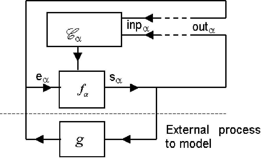
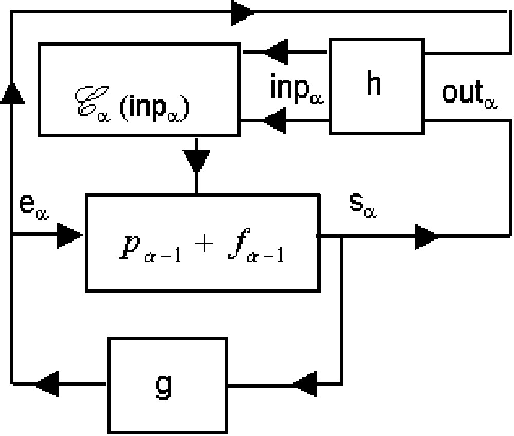
Functioning: M_sp performs the following operations (Fig. 1):

{inp}_{α} = (e_{α}, s_{α}), e_{α}, s_{α} \in \frac{Z}{p Z}

(1)

C_{α} ({inp}_{α}) = f_{α}

(2)

(1) and (2) define the state

S_{α} = (C_{α} ({inp}_{α}), {inp}_{α}) = (f_{α}, {inp}_{α})

s_{α + 1} = f_{α} (e_{α}) = e_{α + 1}

(3)

{out}_{α} = (e_{α + 1}, s_{α + 1}) = (f_{α} (e_{α}), f_{α} (e_{α})) = {inp}_{α + 1}

(4)

(4) defines

F_{α} ({inp}_{α}) = {out}_{α} = {inp}_{α + 1}

(5)

C_{α} ({inp}_{α + 1}) = f_{α + 1}

(6)

The equalities (5) and (6) define the transition function:

δ (f_{α}, {inp}_{α}) = (C_{α} ({inp}_{α + 1}), F_{α} ({inp}_{α})) = (f_{α + 1}, {inp}_{α + 1})

(7)

The recursion

R : C_{α} \mapsto C_{α + 1}

is defined by:

A machine m_sp is thus entirely characterized by the dimensionality of its input space p and its operator ∗.

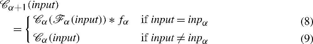
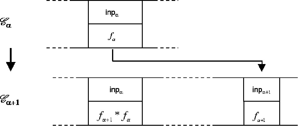
From (5) and (6) and (8), we obtain (Fig. 2):

C_{α + 1} ({inp}_{α}) = C_{α} (F_{α} ({inp}_{α})) * f_{α} = C_{α} ({inp}_{α + 1}) * f_{α} = f_{α + 1} * f_{α}

(8)

2.3 Initialization and trajectory

Initial conditions of a machine m_sp ( $p, *$ ) are given by initial inputs ${inp}_{0}$ and initial function $C_{0}$ :

Initialization

${inp}_{0} = (e_{0}, s_{0})$ and $C_{0}$ are chosen at random at the beginning and once for all from two laws of probability defined respectively by its sample spaces $Inp = \frac{Z}{p Z} \times \frac{Z}{p Z}$ for ${inp}_{0}$ and $P_{A}$ for $C_{0}$ and its uniform distributions:

℘ ({α}) = \frac{1}{p^{2}}, α \in \frac{Z}{p Z} \times \frac{Z}{p Z}

℘ ({f}) = \frac{1}{p^{p}}, f \in P_{A}

Trajectory

The trajectory of m_sp corresponds to successive points $({inp}_{α}, {out}_{α}) \in I \times O$ the machine goes through, starts at $({inp}_{0}, {out}_{0})$ and will be denoted:

Trajectory = {({inp}_{0}, {out}_{0}), \dots, ({inp}_{α}, {out}_{α}), ({inp}_{α + 1}, {out}_{α + 1}), \dots}

Theorem 1

A self-programming machine is a deterministic device, and the cardinality of state set is finite. Therefore such a machine necessarily converges.

Definitions

A m_sp converges whenever a point of its trajectory $({inp}_{τ + n}, {out}_{τ + n})$ is identical to a previous one $({inp}_{τ}, {oup}_{τ})$ . It then indefinitely goes through a limit cycle or n-cycle composed of the n points:

({inp}_{τ}, {out}_{τ}), ({inp}_{τ + 1}, {out}_{τ + 1}), \dots, ({inp}_{τ + n - 1}, {out}_{τ + n - 1}) .

Thus dynamics of m_sp is characterized by the transient length τ and the length n of the limit cycle (i.e. its period).

2.4 Connection to external processes g and h: Machine m_sp1 and m_sp2

In order to show the m_sp adaptive properties:

(1) the m_sp is connected (Fig. 3) to a combinatorial automaton defined by some external function $g \in P_{A}$ . Let us call this machine m_sp1.

1. The equality (3) $e_{α + 1} = s_{α + 1}$ defining the m_sp is replaced by $e_{α + 1}^{'} = g (s_{α + 1}^{'})$ for the m_sp1.

Let us study under which conditions a m_sp that we call m^′_spis identical to m_sp1, i.e. conditions under which a m_sp1 is a self-programming machine m_sp.

The equality (2) $C_{α} ({inp}_{α}) = f_{α}$ defining m_sp is replaced by $C_{α}^{'} ({inp}_{α}) = g ○ f_{α}$ for the m^′_sp.

The equality (6) $C_{α} ({inp}_{α + 1}) = f_{α + 1}$ by $C_{α}^{'} ({inp}_{α + 1}) = g ○ f_{α + 1}$ .

The equality (8) $C_{α + 1} ({inp}_{α}) = C_{α} (F_{α} ({inp}_{α})) * f_{α} = f_{α + 1} * f_{α}$ by $C_{α + 1}^{'} ({inp}_{α}) = C_{α}^{'} (F_{α} ({inp}_{α})) * (g ○ f_{α}) = C_{α}^{'} ({inp}_{α + 1}) * (g ○ f_{α}) = (g ○ f_{α + 1}) * (g ○ f_{α})$ .

Operation ‘○’ is left distributive with ‘∗’, so we can write:

C_{α + 1}^{'} ({inp}_{α}) = g ○ (f_{α + 1} * f_{α})

(9)

In this case:

Theorem 2

m ^′ _sp and m _sp1 are identical and hence have the same trajectory.

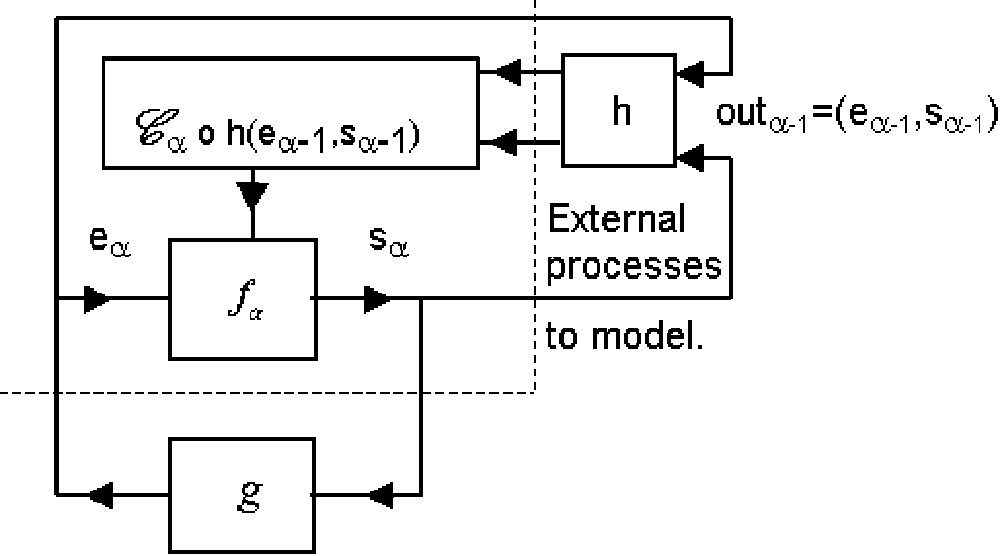
2. M_sp1 is connected (Fig. 4) to another combinatorial automaton defined by any external function $h \in P_{A} \times P_{A}$ . Let us call this machine m_sp2.

The equality (4) ${inp}_{α} = {out}_{α - 1}$ defining the m_sp is replaced by ${inp}_{α}^{″} = h ({out}_{α - 1}^{″})$ for the m_sp2.

Let us study under which conditions a m_sp1 that we call m^″_sp identical to m_sp2:

Then the equality (2): $C_{α}^{'} ({inp}_{α}) = g ○ f_{α}$ defining m_sp1 is replaced by $C_{α}^{″} ○ h ({out}_{α - 1}) = g ○ f_{α}$ for the machine m^″_sp, the equality (6): $C_{α}^{'} ({inp}_{α + 1}) = g ○ f_{α + 1}$ is replaced by $C_{α}^{″} ○ h ({out}_{α}) = g ○ f_{α + 1}$ , and the equality (9) $C_{α + 1}^{'} ({inp}_{α}) = g ○ (f_{α + 1} * f_{α})$ is replaced by $C_{α + 1}^{″} ○ h ({out}_{α - 1}) = g ○ (f_{α + 1} * f_{α})$ .

The function h is injective. In this case:

Theorem 3

m^″_spandm_sp2are identical and hence have the same trajectory.

From now on, we will only study m_sp2 and we call m_sp this machine.

3 Cyclic groups

Let us suppose a m_sp is going through a n-cycle points of which are: ${({inp}_{α}, {out}_{α})}_{α \in I}$ , $I = {τ, τ + 1, \dots, τ + n - 1}$ .

Cyclic group of the states $(G_{S})$

From the equality (7), we can write $S_{α} = (f_{α}, {inp}_{α})$ , $α \in I$ , $δ (S_{α}) = (S_{α + 1})$ , therefore ∃s such as

\underset{s times}{\underset{︸}{δ ○ \dots ○ \partial}} (S_{α}) = (S_{α})

and

(\partial, ○)

generates a cyclic group

G_{S}

order of which is s.

Cyclic group of the n-cycles $(G_{n})$

The function g being fixed at the beginning, one point $({inp}_{α}, {out}_{α})$ of the cycle is only defined by the function $f_{α} : ({inp}_{α}, {out}_{α}) = ((e_{α}, f_{α} (e_{α})), (g ○ f_{α} (e_{α}), f_{α} (e_{α}))$ . If we have a s-cycle for ${(S_{α})}_{α \in I}$ , we obtain an n-cycle for $({({inp}_{α}, {out}_{α}))}_{α \in I}$ with $n ⩽ s$ (hence $n | s$ ).

It therefore depends uniquely on the membership of $f_{α}$ to the equivalence class of polynomials having the same image for the value $e_{α}$ . Therefore the order n of $G_{n}$ is a divisor of s.

4 Conditions of n-cycles

4.1 Linear operator

Definition

In the case of a linear operator ∗, equality (9) becomes: $C_{α + 1} ({inp}_{α}) = f_{α + 1} * f_{α} = λ f_{α + 1} + μ f_{α}$ . For the sake of simplicity, we will simplify this to $C_{α + 1} ({inp}_{α}) = λ f_{α + 1} + f_{α}$ , which not does influence the distribution of n-cycles or transient length.

λ \in \frac{Z}{p Z} - {0} C_{α + 1} ({inp}_{α}) = λ C_{α} ({inp}_{α + 1}) + C_{α} ({inp}_{α}) = λ f_{α + 1} + f_{α}

Let m be the number ( $m ⩽ n$ ) of different input values of the n-cycle. The matrix corresponding to transition from state $(f_{τ + v}, {inp}_{τ + v})$ to state $(f_{τ + v + 1}, {inp}_{τ + v + 1})$ is the $(m \times m)$ matrix:

[\begin{matrix} 1 & \dots & 0 & 0 & \dots & 0 \\ \dots & \dots & \dots & \dots & \dots & \dots \\ 0 & \dots & 1 & λ & \dots & \dots \\ 0 & \dots & 0 & 1 & \dots & 0 \\ \dots & \dots & \dots & \dots & \dots & \dots \\ 0 & \dots & 0 & 0 & \dots & 1 \end{matrix}] [\begin{matrix} f_{τ} \\ \dots \\ f_{τ + v} \\ f_{τ + v + 1} \\ \dots \\ f_{τ + m - 1} \end{matrix}] = [\begin{matrix} f_{τ} \\ \dots \\ f_{τ + v} + λ f_{τ + v + 1} \\ f_{τ + v + 1} \\ \dots \\ f_{τ + m - 1} \end{matrix}]

(10)

The n transitions of the n-cycle give a product

[P]

of n matrices such as:

[P] [\begin{matrix} f_{τ} (e_{τ}) \\ \dots \\ f_{τ + v} (e_{τ + v}) \\ \dots \\ f_{τ + m - 1} (e_{τ + m - 1}) \end{matrix}] = [\begin{matrix} f_{τ + n} (e_{τ}) \\ \dots \\ f_{τ + n + v} (e_{τ + v}) \\ \dots \\ f_{τ + n + m - 1} (e_{τ + m - 1}) \end{matrix}] = [\begin{matrix} f_{τ} (e_{τ}) \\ \dots \\ f_{τ + v} (e_{τ + v}) \\ \dots \\ f_{τ + m - 1} (e_{τ + m - 1}) \end{matrix}]

(11)

Equality (11) implies that the conditions for a m_sp to go through a n-cycle, defined as some vector $[f_{α} (e_{α}), α \in {τ, \dots, τ + m - 1}]$ , is that this vector is an eigenvector associated to eigenvalue 1 of $[P]$ .

Inversely, if we have a product of n ( $m \times m$ ) matrices $[P] = P_{n} . P_{n - 1} . \dots . P_{2} . P_{1}$ where $[P]$ has eigenvalue 1 and $P_{i}$ are matrices such as in the left-hand side of Eq. (10), then we can find a linear m_sp such as these matrices are transition matrices of m_sp and m_spc goes through a n-cycle corresponding to the 1-eigenvector and to the n transition matrices $P_{i}$ .

Theorem 4

A m _sp with linear operator goes through a n-cycle $[f_{α} (e_{α})$ , $α \in {τ, \dots, τ + m - 1}]$ if 1 is an eigenvalue of $[P]$ and $[f_{α} (e_{α}), α \in {τ, \dots, τ + m - 1}]$ its associated eigenvector.

4.2 Polynomial operator

In preliminary unpublished work [39], we have studied the case: $C_{α + 1} ({inp}_{α}) = f_{α + 1} ○ f_{α}$ , where ○ is the composition of functions, thus corresponding to the case where $* = ○$ . We found that, in this case, trajectories always ended in fixed points. We have introduced before the linear case, we now introduce a more general polynomial case.

Definition

A polynomial operator ∗ is defined, for some polynomial $f \in P_{A}$ , by:

C_{α + 1} ({inp}_{α}) = f_{α + 1} * f_{α}

(12)

C_{α + 1} ({inp}_{α}) = C_{α} ({inp}_{α}) + f ○ C_{α} ({inp}_{α + 1}) f \in P_{A}

(13)

C_{α + 1} ({inp}_{α}) = f_{α} + f ○ f_{α + 1}

(14)

We do not have theoretical results in that case and can only give simulations results for such m_sp: all theoretical results presented in the following Sections 5 and 6 only apply to linear machines. Yet, simulations show very similar results for both linear and polynomial operators (see results in §6.1).

5 Association of machines

5.1 Association with a combinatorial automaton

5.1.1 Definition

A combinatorial automaton defined by a function $p_{α \in N} \in P_{A}$ is modified by a m_sp (Fig. 5).

The functioning of this machine (m_spc) differs from a m_sp uniquely by the equality (3) replaced by $s_{α} = p_{α} (e_{α})$ with $p_{α} = p_{α - 1} + f_{α - 1}$ .

In this paper, we consider for simplicity that the functions h and g are identity functions (which implies $e_{α + 1} = s_{α}$ and ${inp}_{α + 1} = {out}_{α}$ ) and the operation ‘∗’ is linear. Apparently, in general case, we cannot obtain theoretical results.

5.1.2 Conditions of n-cycle

Theorem 5

A m _spc goes through a n-cycle if $\forall i, j \in I = {τ, \dots, τ + n - 1}$

– $(f_{i}) (e_{j}) = 0$
– $p_{i} (e_{i}) \neq p_{j} (e_{j})$

Let us suppose this machine goes through a n-cycle, i.e. $α ⩾ τ$ .

We have:

\forall i \in {0, \dots, n - 1}, p_{α + i} (e_{α + i}) = p_{α + n + i} (e_{α + n + i}) = p_{α + 2 n + i} (e_{α + 2 n + i}) = \dots

(15)

We make the demonstration for

i = 0

.

Let P be the matrix defined by the equality (11), let $L_{i}$ be the line vector such as $L_{i} . P$ is the line vector equal to the ith line of P, let V the column vector elements of which are $f_{α} (e_{α}), f_{α + 1} (e_{α}), \dots, f_{α + n - 1} (e_{α})$ , from the equality (15):

p_{α} (e_{α}) = p_{α + n} (e_{α}) gives p_{α} (e_{α}) = p_{α} (e_{α}) + [L_{1} \cdot P] . V

p_{α} (e_{α}) = p_{α + 2 n} (e_{α}) gives p_{α} (e_{α}) = p_{α} (e_{α}) + [L_{1} \cdot P^{2} + L_{1} \cdot P] . V

\dots

p_{α} (e_{α}) = p_{α + n^{2}} (e_{α}) gives p_{α} (e_{α}) = p_{α} (e_{α}) + [L_{1} \cdot P^{n - 1} + \dots + L_{1} \cdot P^{2} + L_{1} \cdot P] . V

which implies

(L_{1} \cdot P) \cdot V = (L_{1} \cdot P^{2}) \cdot V = \dots = (L_{1} \cdot P^{n - 1}) \cdot V = 0

(16)

These n equalities give the following homogenous system:

[\begin{matrix} L_{1} \cdot P \\ L_{1} \cdot P^{2} \\ \dots \\ L_{1} \cdot P^{n - 1} \end{matrix}] V = 0

One obtains by recurrence:

[\begin{matrix} L_{1} \cdot P \\ L_{1} \cdot P^{2} \\ \dots \\ L_{1} \cdot P^{n - 1} \end{matrix}] = [\begin{matrix} 1 & 0 & 0 & 0 & 0 & \dots \\ 1 & λ & 0 & 0 & 0 & \dots \\ 1 & 2 λ & λ^{2} & 0 & 0 & \dots \\ 1 & 3 λ & 3 λ^{2} & λ^{3} & 0 & \dots \\ \dots & \dots & \dots & \dots & \dots & \dots \\ 1 & (\begin{matrix} n - 1 \\ 1 \end{matrix}) λ & (\begin{matrix} n - 1 \\ 2 \end{matrix}) λ^{2} & \dots & \dots & λ^{n - 1} \end{matrix}]

(17)

the determinant of which is equal to

\prod_{i = 0}^{n - 1} λ^{i} = λ^{n (n - 1) / 2} \neq 0

, therefore the only solution of this system is the trivial solution:

f_{α} (e_{α}) = f_{α + 1} (e_{α}) = \dots = f_{α + n - 1} (e_{α}) = 0

.

Repeating the same reasoning for $i = 1, \dots, n - 1$ , the determinant of the system is equal to $\pm λ^{n (n - 1) / 2} \neq 0$ and we obtain

(f_{i}) (e_{j}) = 0

(18)

The equalities

(f_{i}) (e_{j}) = 0

and the equality

e_{α + 1} = [p_{α - 1} + f_{α - 1}] (e_{α})

implies that

\forall i, j ⩾ τ, p_{i} (e_{i}) \neq p_{j} (e_{j})

(19)

The equality

p_{i} (e_{i}) = p_{j} (e_{j})

would imply a cycle of length

n^{'} < n

contrary to the hypothesis (19).

In addition,

p (e_{τ + n - 1}) = e_{τ + n} = e_{τ}

(20)

5.1.3 Distribution of τ and n

Let be given identical machines m_spc differing uniquely by their initial conditions.

Remark

If $℘ ({e}) = \frac{1}{p}$ , $e \in \frac{Z}{p Z}$ , a sequence with elements chosen at random $((e_{α}, e_{α}), (e_{α + 1}, e_{α + 1}), \dots, (e_{α + n - 1}, e_{α + n - 1}))$ can be a trajectory of some m_spc if all the values $e_{i \in α, \dots, α + n - 1}$ are different: $P_{α - 1}$ and $e_{α}$ being given, we have only to choose a function $f_{α - 1}$ that satisfies the equality $f_{α - 1} (e_{α}) = e_{α + 1} - P_{α - 1} (e_{α})$ . We make the same reasoning for the following points of the sequence.

But, if two points in the sequence are equal (for example, $(e_{α}, e_{α})$ and $(e_{α + l}, e_{α + l})$ ), if the value $e_{α + l + 1}$ is such that $e_{α + l + 1} \neq P_{α + l} (e_{α}) + [f_{α} + λ f_{α + 1}] (e_{α})$ , the sequence cannot be the trajectory of a m_spc.

The probability that an arbitrary sequence has all its values different is:

\frac{p - 1}{p} \frac{p - 2}{p} \dots \frac{p - n}{p} = \frac{(p - 1)!}{(p - n - 1)!} \frac{1}{p^{n}},

if n is fixed, this probability tends towards 1 when

p \to \infty

, therefore an arbitrary sequence chosen at random is almost always a trajectory of a m_spc if

p ≫ n

.

Lemma

$℘ [f_{i} (e_{j}) = x] = \frac{1}{p}$ .

The following matrix given in Fig. 6 establishes a one-to-one correspondence between the coefficients of polynomial $f \in P_{A}$ and the values of this polynomial.

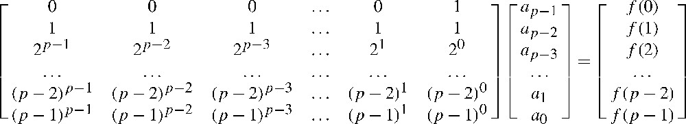
The determinant of this matrix is a Vandermonde determinant equal to $(p - 1)! (p - 2)! \dots 2! 1!$ and different from 0 since p is prime.

The number of functions $f \in P_{A}$ is $p^{p}$ , each function has p coefficients, the number of coefficients of the functions of $P_{A}$ is $p^{p + 1}$ and $\forall x \in \frac{Z}{p Z}$ , $p^{p}$ coefficients are equal to x.

The fact that $p^{p}$ coefficients are equal to x and the correspondence one to one between the coefficients of polynomials $P_{A}$ and the values of these polynomials imply that it exists $p^{p}$ pairs $(i, j)$ such as $f_{i} (e_{j}) = x$ .

Therefore, if the random variable $f_{i}$ and $e_{j}$ have respectively its sample space equal to $P_{A}$ and $\frac{Z}{p Z}$ , and have uniform distributions:

℘ [f_{i} (e_{j}) = x] = \frac{p^{p}}{p^{p + 1}} = \frac{1}{p} .

In the following, we try to find a way to calculate the probability of the event that a m_spc goes through a n-cycle. For that, we should work on the space of all the possible trajectories of m_spc differing by its initial conditions, but it is not a finite space. To get rid of this problem, for fixed n and $p ≫ n$ , we consider just the set $T_{n}$ of all the n-sequence of elements $T_{n} = {((e_{1}, e_{1}), \dots, (e_{n}, e_{n})) | e_{i} \in \frac{Z}{p Z}}$ which is a finite set. In this space, we are looking for the n-cycles. I mean to find a m_spc that goes through these n-elements like a n-cycle. From now on, for n fixed and $p ≫ n$ , as shows our remark, we consider that all elements of $T_{n}$ are on a trajectory of a m_spc which allows us to give the following results:

Let us consider the sequence which elements are chosen at random $((e_{α}, e_{α}), (e_{α + 1}, e_{α + 1}), \dots, (e_{α + n - 1}, e_{α + n - 1}))$ . This sequence corresponds to a n-cycle of m_spc if the three events $f_{i} (e_{j}) = 0$ (18), $p (e_{i}) \neq p (e_{j})$ (19) and $p (e_{τ + n - 1}) = e_{τ}$ (20) occur:

℘ [f_{α} (e_{α}) = 0] = \frac{1}{p} implies ℘ [f_{i} (e_{j}) = 0] = \frac{1}{p^{n^{2}}}, i, j \in I, | I | = n .

We have demonstrated that [35]:

℘ [[p (e_{i}) \neq p (e_{j})] and [p (e_{τ + n - 1}) = e_{τ}]] = \frac{p!}{(n - p)!} . \frac{n}{p^{n + 1}}

The probability that a point in the trajectory of this machine belongs to a n-cycle is the probability that a point belongs to a cycle is:

℘ [E_{n -cycle}] = \frac{1}{n} [\frac{1}{p^{n^{2}}}] . [\frac{p!}{(n - p)!} . \frac{n}{p^{n + 1}}] = ℘ [E_{1-cycle}] + ℘ [E_{2-cycle}] + ℘ [E_{2-cycle}] + \dots = \frac{1}{p^{2}} + \frac{p - 1}{4 p^{6}} + \frac{(p - 1) (p - 2)}{9 p^{12}} + \dots

Now, let us evaluate the probability for a point to be a transient point.

Theorem 6

Under the assumption that the point is in the trajectory of some machine, then obviously:

℘ [transient-point] ≃ 1 - \frac{1}{p^{2}}

and the probability am_spcconverges after τ transient points (the

(τ + 1)

th point is on a cycle) is

℘ (τ) ≃ {(1 - \frac{1}{p^{2}})}^{τ} \frac{1}{p^{2}}

.

τ is a geometric random variable that has expected value $E (τ) = p^{2}$ and variance

E (τ^{2}) - {[E (τ)]}^{2} = 2 p^{4} - p^{2}

The fast convergence of m_spc explains the concordance between the computations and the simulations (Tables 3 and 4).

$\| Input \|$	Expected value of τ: $E (τ)$	Variance of τ: $E (τ^{2}) - {[E (τ)]}^{2}$
	Simulations (linear)	Theoretical value	Simulations (polynomial)	Simulations (linear)	Theoretical value	Simulations (polynomial)
9	9.5	9	8.2	68.8	72	57.5
25	26.6	25	32.9	621.3	600	183.3
49	51.8	49	60.7	2467.6	2352	1214.72
121	125.2	121	132.4	14 974.1	14 520	5528.4

T	\|Input\|=9	\|Input\|=25	\|Input\|=49	\|Input\|=121
Nb of 1-cycles	31,310	31,809	31,916	31,977
Nb of 2-cycles	686	191	84	23
Nb of 3-cycles	4	0	0	0
Frequency of n-cycle n>1	2.15%	0.59%	0.26%	0.07%
$p_{1} / p_{2}$ (simulation)	45.6	166.5	379.9	1390.3
$p_{1} / p_{2}$ (theoretical value)	40.5	156.2	400.1	1464.1

Because of the remark in §5.1.3, notice that for m small enough so that we can find $m - 1$ different points, these $m - 1$ points together with one mth point will be on a trajectory of some m_spc machine. Our assumption is thus very light.

5.2 Association with another $m_{sp}$

Fig. 7a and b shows the two ways of binding together two $m_{sp}$ .

In this paper, we focus on a sequential updating scheme: machines change states one at a time. Other updating regimes (parallel, asynchronous) could also be studied but will not be reported here.

The method to demonstrate the equivalence between one m_sp and a network of n m_sp consists in replacing each term defining one m_sp by a n-tuplet.

For example, in the case of Fig. 7a (Fig. 7b would be similar), equations can be rewritten as:

{inpn}_{α} = ({inp}_{α}, {inp}_{α}^{'}) = ((e_{α}, s_{α}), (s_{α}, e_{α}))

(21)

C n_{α} ({inp}_{α}) = (C_{α} ({inp}_{α}), C_{α}^{'} ({inp}_{α}^{'})) = (f_{α}, f_{α}^{'})

(22)

{outn}_{α} = ((f_{α}^{'} (s_{α}), f_{α} (e_{α})), (f_{α} (e_{α}), f_{α}^{'} (s_{α})))

(23)

{inpn}_{α + 1} = (h ({inp}_{α}), h^{'} ({inp}_{α}^{'}))

(24)

C n_{α + 1} ({inpn}_{α + 1}) = (f_{α + 1} * f_{α}, f_{α + 1}^{'} * f_{α}^{'})

(25)

which shows the equivalence.

6 Results

We now present the results of simulations we have run for $m_{sp}$ machines, linear and polynomial. Each result is obtained by 32 000 simulations of the same machine with different initial conditions chosen at random. $| Input | = p^{2}$ . For each value of p, the machine is chosen at random, i.e. parameter λ for the linear case and polynomial $f \in P_{A}$ are chosen at random.

6.1 $M_{sp}$ with operation ‘∗’ linear and polynomial

The similarity between m_sp with operations ‘∗’ linear and polynomial is striking: we show in Table 2 results of simulations, both for the linear and polynomial cases, indicating that both linear and polynomial cases seem to be in agreement with the theoretical value.

$\| Input \|$	‘∗’ linear	‘∗’ polynomial
	% n-cycle $n \neq 1$	Expected value of τ	% n-cycle $n \neq 1$	Expected value of τ
9	3.28	8.28	3.01	11.82
25	2.63	85.50	1.84	32.92
49	0.55	188.99	0.21	149.46
121	0.052	299.98	0.056	302.34

6.2 $M_{sp}$ associated with a combinatorial automaton

6.2.1 Transient length

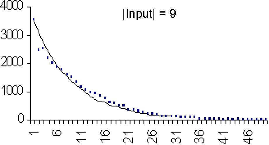
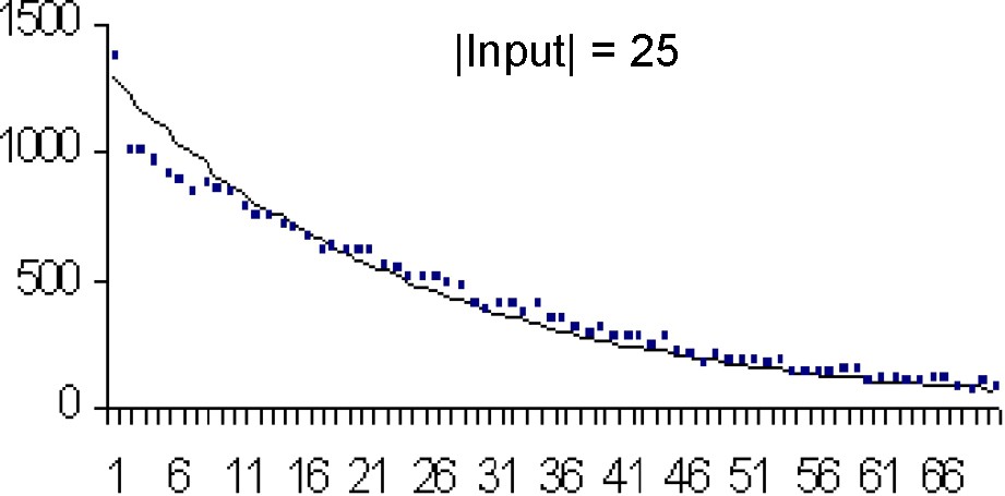
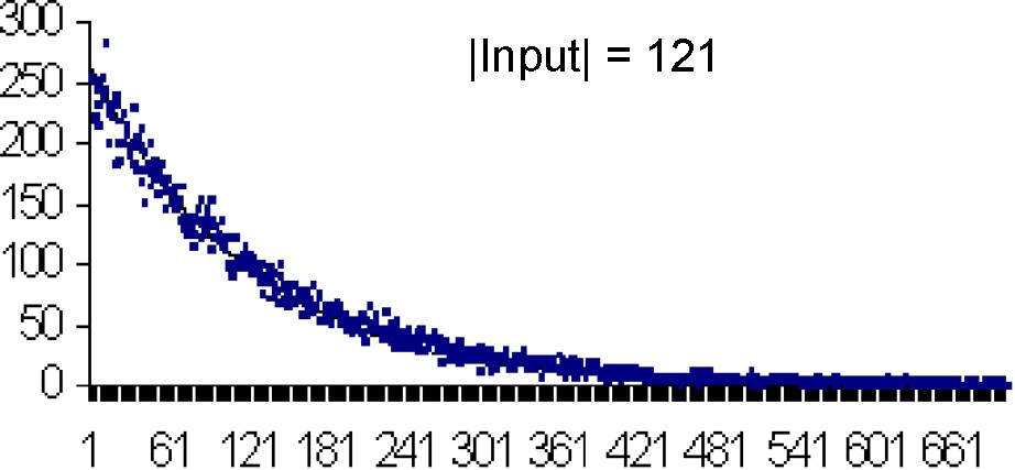
Each figure (Figs. 8–11) compares simulations (points) and computation (theoretical value) from $℘ (τ) ≃ {(1 - \frac{1}{p^{2}})}^{τ} \frac{1}{p^{2}}$ (smooth curve) for a given value of $| Input |$ and for 32 000 simulations, τ is on the X axis, the number of initial conditions on the Y axis.

In Table 3, we compare the mean and variance of τ for different values of $| Input |$ :

6.2.2 Frequency of cycles of length n

Table 4 shows the results of simulations and comparison to the theoretical result obtained in §6.1 for $p_{1} = ℘ (E_{1-cycle}), p_{2} = ℘ (E_{2-cycle})$ . The results show that fixed points (1-cycles) are the most common cycles, and increasingly so with increasing p. Again simulation results are in agreement with the expected theoretical value.

7 Conclusion

We have shown in the two well-known examples of adaptive systems in living beings, the nervous system and the immune system that they share a common property: External signals modify the rewriting of their organization and therefore work as stimuli to modify the ‘program’ of the system.

To get better understanding of this very common feature in the living beings, we have devised the concept of Self-programming machines or m_sp.

These machines have a finite set of inputs, are based on a recurrence and are able to rewrite their internal organization whenever external conditions vary. They have striking adaptation properties:

– they stabilize almost exclusively into 1-cycles;
– the proportion of 1-cycles to all possible n-cycles goes to 1 as the number of inputs increases (i.e. 1-cycles are almost certain);
– they have similar properties whatever the operation defining the recurrence may be (linear or polynomial);
– they will stabilize again in case of small perturbations or intentional massive breakdowns and have proportion of 1-cycles to all possible n-cycles closer to 1 when they are connected in networks.

These results bring us to make the following statement: adaptive properties of living systems can be explained by their ability to rewrite their internal organization whenever external conditions vary under the only assumption that the rewriting mechanism be a deterministic constant recurrence in a finite state set.

References

[1] C. Meyer, Living machines, The New Facts of Life, Wired Magazine, February 2004

[2] H. Von Foerster Cybernetics in circular causal and feedback mechanisms, Transactions of the Sixth Conference, 24–25 March 1949 (H. Von Foerster; M. Mead; H. Teuber; L.J. Macy, eds.), Josiah Macy Jr. Fundation, New York (1949), p. 1

[3] D. Stanley Jones; K. Stanley Jones The Kybernetics of Natural Systems, Pergamon Press, Oxford, UK, 1960

[4] N. Wiener Cybernetics, Hermann, Paris, 1948

[5] P. Glanssdorf; I. Prigogine Structures, Stabilité et Fluctuations, Masson, Paris, 1971

[6] M. Eigen Self-organization of matter and evolution of biological macromolecules, Die Naturwissenschaft, Volume 58 (1971), pp. 463-520

[7] G. Nicolis; I. Prigogine Self-Organization in Nonequilibrium Systems (From Dissipative Structures to Order Through Fluctuations), John Wiley and Sons, New York, 1977

[8] R. Thom Catastrophe Theory, its Present State and Future Perspectives, Dynamical Systems, Lecture Notes in Mathematics, vol. 468, Springer-Verlag, Warwick, 1974

[9] J. von Neumann; A.W. Burks Theory of Self-Reproducing Automata, University of Illinois Press, Urbana, 1966

[10] S. Kaufmann Behavior of randomly constructed genetics nets (C.H. Waddington, ed.), Toward a Theoretical Biology, vol. 3, Edinburgh University Press, Edinburgh, UK, 1970

[11] S. Kaufmann Metabolic stability and epigenesis, Theor. Biol., Volume 22 (1969)

[12] H. Atlan L'Organisation biologique et la Théorie de l'information, Hermann, Paris, 1970

[13] F. Varela Principles of Biological Autonomy, Elsevier/North-Holland, New York/Oxford, 1979

[14] Autopoiesis (M. Zeleny, ed.), A Theory of Living Organization, vol. 3, Elsevier/North-Holland, New York/Oxford, 1981

[15] W.R. Ashby, Principles of self-organizing systems, in: Proc. Western Joint Computer Conf., 1961, pp. 255–278

[16] B.P. Flannery; S.A. Teukolsky; W.T. Vetterling Numerical Recipes, Cambridge University Press, New York, 1986, pp. 326-334

[17] S. Kirkpatrick; C.D. Gelatt; M.P. Vecchi Optimization by simulated annealing, Science, Volume 220 (1983) no. 4598, pp. 671-680

[18] S. Geman; D. Geman Stochastic relaxation, Gibbs distribution and the Bayesian restoration of images, IEEE Trans. PAMI, Volume 6 (1984), pp. 721-741

[19] D.D. Rumelhart; G.E. Hinton; R.J. William; R.J. Learning Representations by back-propagating errors, Nature, Volume 323 (1986), pp. 533-536

[20] P. Gallinari; S. Thiria; F. Badran; F. Fogelman-Soulié On the relations between discriminant analysis and multilayer perceptrons, Neural Networks, Volume 4 (1991), pp. 349-360

[21] L.J. Fogel; P.J. Angeline; D.B. Fogel An evolutionary programming approach to self-adaptation on finite states machines, Evol. Program. (1995), pp. 355-365

[22] R. Forsyth A Darwinian approach to pattern recognition, Kibernetes, Volume 10 (1981), pp. 159-166

[23] S. Haykin, Adaptive Filter Theory, third ed., Prentice-Hall, Neurol. Zentralbl. 34 (1996) 338

[24] A. Benvéniste; M. Goursay; G. Ruget Robust identification of a non-minimum phase system: Blind adjustement of a linear equalizer in data communications, IEEE Trans. Autom. Control, Volume 3 (1996), pp. 385-399

[25] A. Marina Die Relationnen des Palaeencephalons sind nicht fix, Neurol. Zentralbl., Volume 34 (1915), p. 338

[26] R.W. Sperry Effects of crossing nerves to antagonistic limbs muscles in the monkey, Arch. Neurol. Psychiatry, Volume 58 (1947), p. 542

[27] T.J. Wills; C. Lever; F. Cacucci; N. Burgess; J. O'Keefe Attractor dynamics in the hippocampal representation of the local environment, Science, Volume 308 (2005) no. 5723, pp. 873-876

[28] H. Eisen Immunology, Harperand Row, New York, 1980

[29] D. Dasgupta, Artificial Neural Networks and Artificial Immune Systems: Similarities and Differences, in: Proc. Int. Conf. on Systems, Man and Cybernetics, Orlando, FL, USA, 12–15 October 1997

[30] A. Perelson; G. Weisbuch Immunology for physicists, Rev. Mod. Phys., Volume 69 (1997) no. 4

[31] L. Hodgkin; A.F. Huxley A quantitative description of membrane current and its application to conduction and excitation in nerve, J. Physiol., Volume 117 (1952), pp. 500-544

[32] D.O. Hebb The Organization of Behavior, A Neuro-Psychological Theory, Wiley, New York, 1949

[33] W.S. McCulloch; W. Pitts A Logical Calculus of the Ideas Immanent in Nervous Activity, Bulletin of Mathematical Biophysics, vol. 5, 1943, pp. 115-133

[34] K. Abbas; A.H. Lichtman Basic Immunology, Functions and Disorders of the Immune System, Saunders imprint of Elsevier, 2004

[35] P. Dumouchel; J.-P. Dupuy Colloque de Cerisy, L'auto-organisation, Seuil, Paris, 1983

[36] J.-P. Moulin Modifiable automata, Self-modifying automata, Acta Biotheor., Volume 40 (1992) no. 2/3, pp. 195-204

[37] Y. Bar-Yam Dynamics of Complex Systems, Addison-Wesley, 1997

[38] W.R. Ashby Design for a Brain, Chapman and Hall, London, 1952

[39] J.-P. Moulin, Self-Programming Machines I, Unpublished, 2000

Comments - Policy

1 Introduction

2 Self-programming machines. Description and functioning

2.1 Components

2.2 Definition and functioning

Definition

2.3 Initialization and trajectory

Initialization

Trajectory

Theorem 1

Definitions

2.4 Connection to external processes g and h: Machine msp1 and msp2

Theorem 2

Theorem 3

3 Cyclic groups

Cyclic group of the states (GS)

Cyclic group of the n-cycles (Gn)

4 Conditions of n-cycles

4.1 Linear operator

Definition

Theorem 4

4.2 Polynomial operator

Definition

5 Association of machines

5.1 Association with a combinatorial automaton

5.1.1 Definition

5.1.2 Conditions of n-cycle

Theorem 5

5.1.3 Distribution of τ and n

Remark

Lemma

Theorem 6

5.2 Association with another msp

6 Results

6.1 Msp with operation ‘∗’ linear and polynomial

6.2 Msp associated with a combinatorial automaton

6.2.1 Transient length

6.2.2 Frequency of cycles of length n

7 Conclusion

2.4 Connection to external processes g and h: Machine m_sp1 and m_sp2

Cyclic group of the states $(G_{S})$

Cyclic group of the n-cycles $(G_{n})$

5.2 Association with another $m_{sp}$

6.1 $M_{sp}$ with operation ‘∗’ linear and polynomial

6.2 $M_{sp}$ associated with a combinatorial automaton