1 Introduction
The vast majority of the methods used until now to compare genomes have been based upon techniques of local alignment of two or more DNA or protein sequences. These methods are very successful for phylogenetic studies of gene/protein families or superfamilies and even for the phylogenies of complete genomes when the evolutionary divergence is not too great.
Alignment-free methods are rarely used in biology, although they can be quite successful in linguistic studies [1]. Their actual name in the literature can differ; they are referred to variously as n-grams, n-words, or k-tuples. However, they all describe the same concepts and approaches, namely the analysis of occurrences in a text, of words of various lengths and containing n letters. For , the words can be called bigrams. This is the term I shall use in this article. One can find a more exhaustive description of various alignment-free methods in recent reviews [2,3].
Forty years ago, A. Krzywicki and I introduced, for the first time, the bigram analysis of biological texts, namely the texts of the very few protein sequences available in the 1960s [4,5]. We developed the notion of the expectancy-rectified frequencies of pairs of amino acids, in other terms bigrams, with spacer (s) – i.e. the observed frequency of occurrence of the s-pair of amino acids , compared to the expected frequency of such s-pair occurrence []. We have shown that, for certain spacer lengths, statistically highly significant deviations could be observed, and we speculated that these deviations were due to spatial constraints in the structure of biologically active proteins. This work had a certain success, since it is quoted in a recent history of bioinformatics among the few articles germane as precursors of this scientific discipline in its ‘protohistorical’ era [6]. It was, at the same time, a total failure, since nobody has followed up or developed our approach. More than thirty years later, Radomski and I used, to a small extent, the bigram analysis to develop the notion of the genomic style of proteins [7], and more recently to examine the primary sequences of proteins from 52 species [3]. In this latter work, we have shown that amino acid sequences of complete proteomes display a singular periodicity around 3.5 polypeptide bonds. We hypothesized that the oscillations observed at the level of whole proteomes may result from the periodic nature of the alpha-helical proteins, which have, as it is well known, the same basic frequency.
In the present work, I have applied the expectancy-rectified frequency of bigrams to the study of the DNA from 80 completely sequenced procaryotic genomes. I show that all genomes display highly significant periodic oscillations with a period of 11 phosphodiester bonds, and that these oscillations result from the presence of open reading frames coding for alpha-helical proteins. The period of 11 phosphodiester bonds is in perfect agreement with the period of 3.5 for polypeptide bonds.
Unexpectedly however, the amplitude of nucleotide sequence oscillations in genomes can differ dramatically from one bacterial species to another. Furthermore, sets of homologous and very similar genes from different organisms can display drastically different oscillations. I conclude with a heterodox idea that very similar proteins having the same biochemical function and the same ancestor either may have different secondary structures or may use different ways to be constructed.
2 Materials, symbols and methods
2.1 Materials
All genomic nucleotide sequences were retrieved from the Comprehensive Microbial Resource (CMR) Data Base of the Institute for Genomic Research (http://www.tigr.org) [8] in February 2005, with their original annotations. Chromosomes but not plasmids were retrieved. All data concerning the structure of proteins were retrieved from RCSB Protein Data Bank using its mirror site (http://www.pdb.mdc-berlin.de/pdb) in September 2005, and the nucleotide sequences corresponding to the coding sequences for these proteins were retrieved from the EMBL-EBI (http://www//.ebi.ac.uk/Databases/). In every case, I have verified that the translation of the EBI coding sequence was identical to the fasta protein sequence given in PDB. This was essential since, in a number of cases, the data from the two databases were contradictory.
2.2 Symbols and methods
The general way of presenting the data will be the symbol , where B is the number of bigram occurrences in a sequence, d is the distance (in number of phosphodiester bonds) separating the two terminal nucleotides and k is the kind of association of the terminal nucleotides studied. There are 16 kinds of bigrams: AA, AG, AT, AC, GA, GG, GT, GC, TA, TG, TT, TC, CA, CG, CT, and CC.
Notice that the actual length of oligonucleotides analysed is equal to (), e.g., corresponds to the complete set of all dodecanucleotides beginning with A (adenine) and terminating with C (cytosine), independently of the nature of nucleotides between A and C. Furthermore, is different from because of the 5′ to 3′ polarity of the polynucleotide chain. When necessary, the abbreviation of the genome analysed is given, e.g., HelPy corresponds to all such dodecanucleotides from the genome of Helicobacter pylori (for the list of abbreviations, see Table 1).
Notice that:
- – (i) each nucleotide in a certain position of the sequence is represented 400 times in the sum total of bigrams, e.g., a given C in a position p is represented, on the one hand, in 200 oligonucleotides having Cytosine at the 5′ end and terminating by anyone of the four nucleotides at the 3′ end (symbolized by ) and, on the other hand, the same C at the same position is represented in 200 oligonucleotides having A, G, C or T at the 5′ terminus and a Cytosine at the 3′ end (symbolized by );
- – (ii) the sum total of all bigrams counted in a nucleotide sequence of a length L is equal to . For example, in Helicobacter, where , this sum is 335 204 484, while for an average ORF of , the sum is 180 699. The total number of bigrams analysed in all 80 genomes is (see Table 1 for the complete dataset).
The computer program, written by Joël Prince in the ‘4th dimension’ software for a PC, counts all the 16 kinds of bigrams from to in about an hour for a genome of a few million nucleotides. These counts are symbolised as for the observed occurrences. They will be compared to the , the expected values computed on the basis of the null hypothesis, i.e. a random association of nucleotides. The values are calculated as a product of the frequencies of single nucleotides A, G, T and C in the oligonucleotide segment analysed, for each different d value. Notice that the values are practically identical for all the different d values in the case of very long nucleotide sequences, such as those of complete genomes, while they may be quite different for much shorter sequences such as the individual protein coding sequences (ORFs, Open Reading Frames). In this latter case, the and numbers are calculated separately for every individual ORF and summed, if necessary. In this way, it is possible to build up a representation of the complete proteome of a species, or a subset of ORFs from it. Excel was used for other calculations.
To facilitate the comparisons, the sizes of the various genomes were normalized to one Genome Unit Size, GUS (one GUS = 500 000 nucleotides). This normalization consists in multiplying all the values computed for the whole genome by a normalization factor: 500 000/the size of the genome in nucleotides. The smallest genome analysed, Nanoarchaeum equitans, has a size close to 1 GUS.
3 Results and discussion
3.1 Raw data
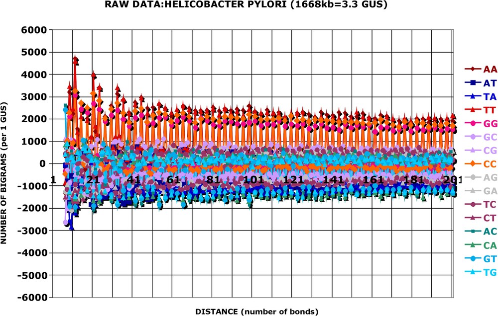
The main purpose of this study is to analyse the differences between the observed bigrams and those predicted by the null hypothesis. The computer programme calculates these differences, – , for every separate d, separate k and separate genome. These values will be referred to as raw data, , and are plotted as a function of d. Three examples are shown in Fig. 1 (and Figs. A1–A21), and several others are available in the supplementary material.
The inspection of the raw data discloses, first of all, a striking and easy to interpret feature. There is a phase given by three phosphodiester bounds in the frequency of bigrams. This phase is more easy to perceive in the kinds of bigrams that protrude from the central mass like AA, TT, GG, CC, on one hand, or AC, CA, GT, TG, on the other hand. It is obvious that this phasing corresponds to the reading frames of the protein coding sequences (ORFs), which represent most of the nucleotide sequence in all procaryotic genomes. The eight above-mentioned kinds of bigrams present maximum deviations in the reading frame zero, i.e. at bond distances that are multiples of 3 (see Fig. 1 and Table 3 – and Figs. A1 and A2). I have verified that this depends neither on the (G + C) content of the genome nor on the amino acid composition of the proteome. It is the case with all genomes analysed. Thus, the frequencies, which relate the first position of a codon with the first position of another codon (the second position with the second position and the third with the third), some 99 or 198 phosphodiester bonds further down are the most strongly deviating from random (see Tables 2 and 3 for more explanations). The fact that the ORFs are not in phase on the same DNA strand, on the one hand, and that, on the other hand, the nucleotide sequence analysed is the Watson strand only, while the ORFs can be (and most frequently are) located on both strands, does not influence the issue. Since the programme scans the distances smaller than 201, and the average size of an ORF is close to 900, the majority of bigram occurrences counted is located inside the ORFs and not outside or between them. This argument becomes even stronger when one considers that the most interesting deviations from randomness occur at distances smaller than 50 phosphodiester bonds (see below).
The differences () between the observed number of occurrences () and the expected number of occurrences () was calculated for the complete nucleotide sequence of the genome and the resulting values were normalised to 1 GUS by the coefficient 500 000/1 551 335. For each kind of bigram, one obtains 192 values of corresponding to distances from d=5 to d=196. These values are grouped into four successive quarters of the total distance and summed up separately for the three Reading Frames (see Table 2). In each Reading Frame and for each kind of bigram, there are 16 values of , the sum of which is given in black (e.g., ). For the same 16 values, one calculates the variance, which is shown in bold, as standard deviation (std, σ) of the mean (e.g., 56 195/16=3512, σ=966 for the Reading Frame 0 of ). The sum total of is of course 0 and the sum of standard deviations gives an estimate of the total variance. Some kinds of bigrams are always overrepresented ( are positive, e.g., AA, TT), some are always underrepresented ( are negative, e.g., AT, TA), whatever the Reading Frame and whatever the distance. This observation is true for all the genomes analysed. For other kinds of bigrams, the +1 Reading Frame occurrences are overrepresented and the −1 Reading Frame occurrences are underrepresented (e.g., GT or GA), while the converse is true for TG and CA. The difference of occurrences (measured by the sum of the three frames) decreases systematically from the first quarter to the last quarter for the bigrams AA, AT, TA, TT, GG, CC, AC, CA, GT, TG (again this observation is true for all the genomes analysed), while such a decrease is not systematically observed for the remaining six bigrams and depends on the genome studied. The first quarter of distances is singular in several respects: (i) its total variance is significantly greater than that of the next quarters (4 to 6 times greater in any one of the genomes analysed), (ii) the variance of the Reading Frame 0 is greater than that of the two other Reading Frames, while this is not the case for the next quarters where the three Reading Frames contribute about 1/3 of variance each, (iii) different kinds of bigrams contribute unequally to the total variance in the first quarter (e.g., the bigrams AA, AT, TA and TT contribute each 10 to 12%, while the bigrams AG, GA, TC and CT contribute each 4 to 5%), while this is not the case for the last quarters, where each kind of bigrams contributes roughly 6% of the total variance. Fig. A3 summarizes the results in a graph and Figs. A4 and A5A give examples for other genomes. In order to make the oscillations of the first quarter more conspicuous, the average background occurrences of the last two quarters are subtracted in phase from those of the first quarter: , (, etc. After this subtraction, referred to as ‘pruning’ and symbolized by , about 90% of total variance results from variations in the number of occurrences located in the first quarter (see Fig. A5B)
| An example of bigram occurrences: complete genome of Aquifex aeolicus (1551335 nucl.) normalised to 1 GUS | |||||||||||||||||||||
| Difference in the number of occurrences | |||||||||||||||||||||
| Variance analysis of occurrences( std=standard deviation of the mean) | |||||||||||||||||||||
| Distance (fraction of total) | Distance (number of bonds) | AA | AT | TA | TT | GG | GC | CG | CC | AG | GA | TC | CT | AC | CA | GT | TG | SUM 16 KINDS OCCURRENCES | SUM 16 STD | TOTAL VARIANCE | |
| Reading Frame 0 | first quarter | sum (d=6+9+12+⋯+51) | 56 195 | −12 380 | −13 831 | 58 461 | 55 113 | −8712 | −9827 | 51 870 | 1820 | 1550 | 2478 | 1869 | −45 636 | −43 912 | −47 941 | −47 116 | 0 | ||
| Reading Frame +1 | first quarter | sum (d=7+10+13+⋯+52) | 21 424 | −19 889 | −31 682 | 19 292 | −6520 | −20 556 | 20 024 | −3804 | −1038 | 23 209 | 24 858 | −3271 | −499 | −12 950 | 3877 | −12 477 | 0 | ||
| Reading Frame −1 | first quarter | sum (d=5+8+11+⋯+50) | 21 710 | −31 440 | −23 908 | 20 290 | −6626 | 21 214 | −22 928 | −5007 | 23 522 | −447 | −2412 | 25289 | −13 794 | 2646 | −14 131 | 6021 | 0 | ||
| Sum three frames | first quarter | total | 99 329 | −63 709 | −69 421 | 98 042 | 41 968 | −8054 | −12 731 | 43 059 | 24 304 | 24 312 | 24 925 | 23887 | −59 929 | −54 216 | −58 195 | −53 572 | 0 | ||
| Reading Frame 0 | first quarter | std () | 966 | 1158 | 801 | 965 | 321 | 152 | 229 | 352 | 402 | 281 | 286 | 398 | 382 | 426 | 350 | 404 | 7873 | ||
| Reading Frame +1 | first quarter | std () | 511 | 378 | 472 | 451 | 153 | 152 | 232 | 172 | 204 | 239 | 276 | 269 | 367 | 289 | 370 | 314 | 4849 | ||
| Reading Frame −1 | first quarter | std () | 636 | 677 | 591 | 664 | 184 | 195 | 142 | 192 | 284 | 286 | 282 | 174 | 320 | 327 | 284 | 329 | 5567 | ||
| Sum three frames | first quarter | total | 2113 | 2213 | 1864 | 2080 | 659 | 499 | 603 | 716 | 890 | 805 | 844 | 841 | 1069 | 1042 | 1004 | 1047 | 18 289 | ||
| Reading Frame 0 | second quarter | sum (d=54+57+60+⋯+99) | 50 049 | −14 616 | −12 550 | 52 403 | 48 644 | −8679 | −10 209 | 45 529 | 3724 | 1536 | 2302 | 3718 | −39 166 | −39 025 | −41 475 | −42 185 | 0 | ||
| Reading Frame +1 | second quarter | sum (d=55+58+61+⋯+100) | 16 741 | −18 965 | −29 225 | 15 314 | −8304 | −20 382 | 18 414 | −5863 | −110 | 22 788 | 23 905 | −2242 | 2326 | −10 296 | 5923 | −10 024 | 0 | ||
| Reading Frame −1 | second quarter | sum (d=53+56+59+⋯+98) | 16 556 | −28 184 | −18 560 | 15 367 | −6890 | 19 666 | −21 704 | −5892 | 22 434 | −1712 | −2973 | 23 887 | −10 815 | 3724 | −11 039 | 6135 | 0 | ||
| sum three frames | second quarter | total | 83 347 | −61 765 | −60 335 | 83 084 | 33 450 | −9396 | −13 499 | 33 775 | 26 047 | 22 612 | 23 235 | 25 363 | −47 656 | −45 597 | −46 592 | −46 073 | 0 | ||
| Reading Frame 0 | second quarter | std () | 122 | 153 | 127 | 110 | 79 | 99 | 91 | 72 | 78 | 87 | 132 | 115 | 93 | 71 | 110 | 134 | 1671 | ||
| Reading Frame +1 | second quarter | std () | 109 | 123 | 71 | 90 | 105 | 104 | 111 | 84 | 145 | 86 | 95 | 121 | 63 | 95 | 76 | 87 | 1565 | ||
| Reading Frame −1 | second quarter | std () | 114 | 126 | 83 | 137 | 111 | 68 | 83 | 76 | 120 | 76 | 85 | 100 | 89 | 71 | 92 | 121 | 1552 | ||
| sum three frames | second quarter | total | 345 | 401 | 281 | 337 | 295 | 272 | 284 | 232 | 342 | 249 | 311 | 336 | 245 | 237 | 278 | 343 | 4787 | ||
| Reading Frame 0 | third quarter | sum (d=102+105+108+⋯+147) | 46 405 | −14 772 | −11 781 | 48 706 | 44 894 | −9511 | −9239 | 42 414 | 4227 | 2798 | 2952 | 4251 | −35 880 | −37 402 | −38 149 | −39 914 | 0 | ||
| Reading Frame +1 | third quarter | sum (d=103+106+09+⋯+148) | 16 138 | −17 886 | −27 349 | 15 178 | −7049 | −19036 | 17 037 | −4872 | 240 | 21 369 | 22 396 | −2005 | 1488 | −10 138 | 4750 | −10 262 | 0 | ||
| Reading Frame −1 | third quarter | sum (d=101+104+107+⋯+146) | 15 761 | −26 263 | −17 238 | 15 328 | −5893 | 18 846 | −20572 | −4791 | 21 519 | −1084 | −3042 | 22 809 | −11 037 | 2579 | −11 836 | 4913 | 0 | ||
| sum three frames | third quarter | total | 78 304 | −58 920 | −56 368 | 79 212 | 31 952 | −9701 | −12 775 | 32 751 | 25 986 | 23 083 | 22 306 | 25 055 | −45 428 | −44 960 | −45 235 | −45 263 | 0 | ||
| Reading Frame 0 | third quarter | std () | 134 | 79 | 110 | 125 | 53 | 76 | 76 | 104 | 52 | 82 | 86 | 95 | 94 | 103 | 67 | 103 | 1438 | ||
| Reading Frame +1 | third quarter | std () | 76 | 89 | 77 | 84 | 84 | 96 | 87 | 66 | 82 | 68 | 49 | 62 | 88 | 74 | 92 | 83 | 1255 | ||
| Reading Frame −1 | third quarter | std () | 86 | 75 | 93 | 100 | 69 | 93 | 61 | 70 | 91 | 108 | 78 | 98 | 61 | 98 | 65 | 87 | 1333 | ||
| Sum three frames | third quarter | total | 297 | 243 | 279 | 309 | 206 | 266 | 223 | 240 | 225 | 258 | 213 | 254 | 243 | 275 | 224 | 274 | 4027 | ||
| Reading Frame 0 | fourth quarter | sum (d=150+153+156+⋯+195) | 43 282 | −14 676 | −10 744 | 45 730 | 42 139 | −9097 | −8561 | 39 111 | 3566 | 2564 | 2169 | 4540 | −32 202 | −35 072 | −35 561 | −37 189 | 0 | ||
| Reading Frame +1 | fourth quarter | sum (d=151+154+157+⋯+196) | 15 145 | −18 081 | −25 697 | 14 011 | −7820 | −17 499 | 15 847 | −5149 | 1456 | 20 509 | 21 179 | −752 | 1450 | −9927 | 4855 | −9526 | 0 | ||
| Reading Frame −1 | fourth quarter | sum (d=149+152+155+⋯+194) | 15 429 | −25 656 | −16 732 | 14 448 | −5252 | 16 809 | −19 834 | −4233 | 20 141 | −1001 | −2649 | 21 750 | −9944 | 2334 | −10 510 | 4900 | 0 | ||
| Sum three frames | fourth quarter | total | 73 855 | −58 412 | −53 173 | 74 190 | 29 067 | −9788 | −12 548 | 29 729 | 25 163 | 22 071 | 20 699 | 25 538 | −40 695 | −42 665 | −41 216 | −41 816 | 0 | ||
| Reading Frame 0 | fourth quarter | std () | 108 | 96 | 94 | 101 | 104 | 63 | 82 | 103 | 80 | 70 | 96 | 91 | 101 | 126 | 74 | 96 | 1487 | ||
| Reading Frame +1 | fourth quarter | std () | 104 | 110 | 114 | 78 | 79 | 70 | 85 | 61 | 65 | 85 | 94 | 95 | 63 | 83 | 90 | 70 | 1348 | ||
| Reading Frame −1 | fourth quarter | std () | 78 | 94 | 105 | 112 | 64 | 77 | 77 | 74 | 93 | 97 | 68 | 89 | 75 | 88 | 93 | 84 | 1366 | ||
| Sum three frames | fourth quarter | total | 289 | 300 | 312 | 291 | 246 | 210 | 244 | 239 | 238 | 253 | 258 | 275 | 240 | 298 | 257 | 251 | 4201 |
This example (which can be verified without computer) illustrates how the number of occurrences of bigrams observed () is counted and how the number of occurrences of bigrams expected () is calculated (e.g., for ). Obviously, in this example, the difference between the observed and expected occurrences is not statistically significant. For examples of statistically significant data, see Table 3 and Fig. 5 and Figs. A13–A16. In procaryotic genomes, the majority of bigrams for distances (d) below 201 (and a fortiori for d below 50) belong to one and the same ORF (Open Reading Frame, a putative protein-coding sequence), and not to an intergenic region or to two successive ORFs (whether located on the same DNA strand or on opposite strands), for two reasons: (i) the average length of an ORF is around 900 nucleotides and (ii) the average length of protein coding sequences is close to 90% of the total genomic length. Therefore, the bigrams corresponding to distances, d, which are multiples of three (i.e. 6,9,12…) will be referred to as Reading Frame 0, while other bigrams will be referred to as Reading Frame +1 or −1. This distinction is important as it is apparent from the data calculated on a real genome (see Table 3)
The second feature, as prominent as the first one and directly related to it, is not as obvious to interpret at its face value. It concerns the direction of changes. It is apparent that bigrams of the first group (AA, TT, GG, CC) are always over-represented, while those of the second group (AC, CA, GT, TG) are always under-represented in the reading frame zero: the maximum positive points are red (see Fig. 1 and Figs. A1 and A2), while the minimal negative points are blue all along the distance axis (Fig. 1, Table 3, and Figs. A1 and A2). This observation is, once more, true for all genomes. Finally, the variations of the remaining eight kinds of bigrams, which also depend on the reading frame, are less conspicuous (Table 3) and more variable from one genome to another. The in-depth analysis of changes related to the reading frame is not the aim of the present article and will be presented elsewhere (Slonimski, in preparation).
To eliminate the reading frame parameter, I have recalculated the raw data, as in Fig. 1 and Figs. A1 and A2, by a sliding window of three successive values, beginning with . Such smoothed data correspond, in succession, to the average of … and are centred at , , , etc. In this way, the occurrences of bigrams in the three reading frames are averaged, since is in the frame −1, is in the frame 0 and in the frame +1. All successive bigrams are averaged in the same manner.
The second calculation, which is another way to the main issue of this study, is even simpler. I observed that the amplitude of the reading frame oscillations of the raw data is more heterogeneous for the small distances, from to , than for the much larger distances. This effect appears to be small but can be easily detected in Fig. 1, while it is not as conspicuous in Figs. A1 and A2 of the raw data. However, it can be demonstrated in all genomes and it is explained in details in Table 3. Figs. A3–A5 show the results of a variance analysis along the distance axis. I have calculated the standard deviations for four sets of the values in the same reading frame and separately for each quarter of the total nucleotide length examined. Each quarter (for the first quarter: bonds for the reading frame 0; bonds for the reading frame +1; bonds for the reading frame −1; for the other quarters, see the abscissas of Figs. A3–A5 and Table 3) gives 16 values of standard deviations, which are summed to estimate the total variance. In all genomes examined and in every reading frame, the variance is much greater for the first quarter, i.e. short distances d, than for the last quarters (long distances d). Three examples are shown in Figs. A3–A5 and others can be consulted in the supplementary material. Furthermore, the variance of the last two quarters is always the same. In other words, there is a novel source of heterogeneity of values occurring at distances from 5 to 52 bonds, which is superimposed on a constant background resulting from the reading frame effects. To make this novel source of heterogeneity more conspicuous, I have subtracted, in phase, from the values of the first quarter an average of the two last quarters: , , , etc. This subtraction and the sliding window operation transform the raw data into ‘pruned’ (symbolized as ) data, which allows the main conclusions of this work to be deduced. Fig. A5B shows that the pruned data make the oscillations of the first quarter more conspicuous and significant.
3.2 Pruned data
The main results are straightforward and are given in a series of figures (Figs. 2–4 and Figs. A6–A12). They show that the frequency of bigrams in a genome varies in a regular and periodic manner as a function of the number of bonds separating the two terminal, 5′ and 3′, nucleotides in the span of distances between 6 and 51 nucleotides. This periodicity is not due to the reading frame effects discussed above, since we are dealing here with the pruned data.
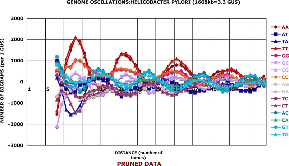
Pruned data: Helicobacter Pylori. The numbers of bigram occurrences shown in Fig. 1 were ‘pruned’ by subtraction in phase as explained in Table 3 and averaged by the sliding window of three successive values: ; , etc. and plotted as a function of the average distance .
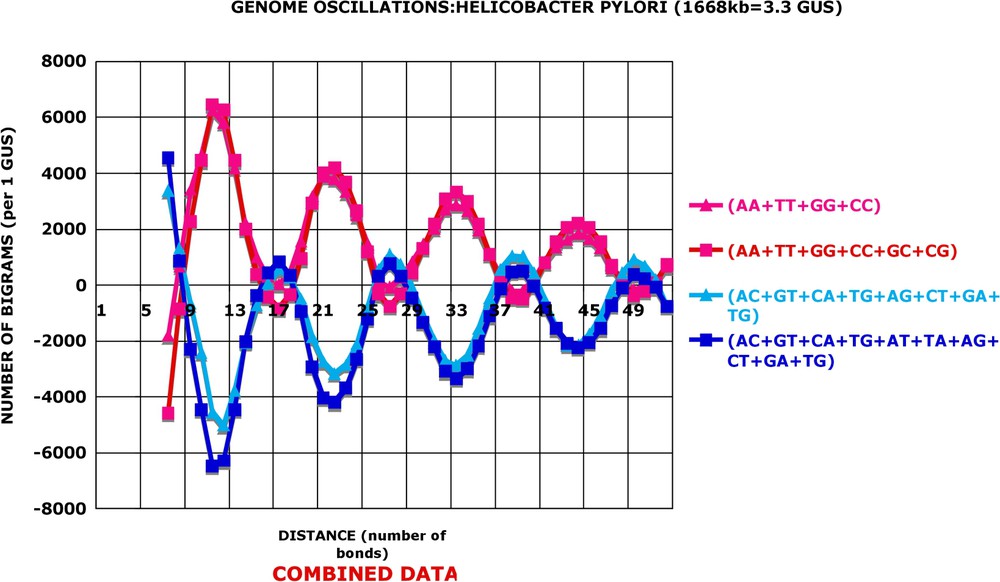
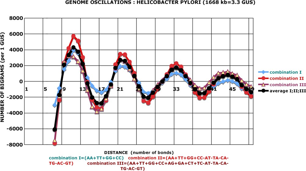
Combined data: Helicobacter pylori. The data of Fig. 2 were combined by adding, as indicated, the different kinds of pruned and averaged numbers of bigram occurrences and plotted as in Fig. 2. , etc.
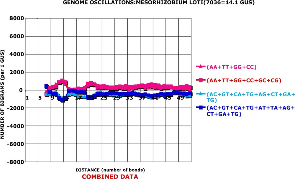
Combined data: Mesorhizobium loti. As in Fig. 3.
In Fig. 2, one can see that the various kinds (parameter k) of bigrams vary either in conjunction with each other (e.g., or are both very high for and , high for and , and moderately high for and , etc.) or in opposition (for the same values of d, the bigrams or display negative frequencies). In other terms, the associations AA or TT are more abundant than random for distances 11 and 12, while the associations TA or TG are less abundant than random for the same distances. The oscillations of frequencies along the distance axis are even more striking when one groups together various kinds of bigrams, as shown in Fig. 3. In this figure, I have added the numbers of bigrams of different kinds in various combinations, e.g., . It is apparent that the positive, over-represented oscillations become stronger after grouping as well as the negative, under-represented ones (e.g., ). Finally, the oscillations of the Helicobacter pylori genome appear with a regular periodicity: the average period for the positive oscillations is 10.9 bonds and the average period for the negative ones is not distinguishable from it, i.e. 10.8 bonds.
These observations immediately raise a number of questions. I shall try to answer a few of them:
- – (i) what is the statistical significance of the results observed?
- – (ii) how general is the presence of periodic oscillations? Is it different either in amplitude or in the period itself for different species? If so, how is it related to their phylogeny and evolution, or to some other overall properties of genomes, such as their size or their (G + C) content?
- – (iii) there are 16 kinds of bigrams, which can be grouped or combined in many different ways. Is there a simple way to describe the oscillations? In other terms, is there a unique combination, or a small number of combinations, which could lead to the most germane description of all genomes on one hand, and to the most pertinent discrimination between genomes on the other?
- – (iv) finally, what is the origin or cause of the periodic oscillations of the nucleotide sequences of genomes?
The answer to the first question is simple. All interesting results are statistically significant. Although the amplitude of oscillations may appear quite small in terms of percentages of the total number of bigrams analysed (e.g., the excess of bigrams AA at the distance of 11 bonds is equal to 2079 in the total of 499 989 bigrams counted for 1 GUS of Helicobacter, i.e. 0.4%, see Fig. 2), its statistical significance is huge. I have performed a Khi2 analysis of conformity between the observed and the expected bigrams. To this end, I have calculated the Khi2 for each d and each k and plotted them as a function of d. In addition, I have calculated the Khi2 for various combinations of individual k, e.g., and . The rationale of this approach is straightforward. If the oscillations are in the same phase, then the Khi2 for should be always much greater than for . If the oscillations are in opposite phases, then the Khi2 of the difference should be greater than the Khi2 of the sum. A few examples are given in Fig. 5 and Figs. A12–A16, where each point has one degree of freedom. The probability that the 0.4% excess of B11AA is due to chance is equal to for 1 GUS of Helicobacter and 10−52 for its true genome size of 1668 kb. This is one of the major advantages of working with the complete genomes: very small variations become highly significant because of the large numbers involved.
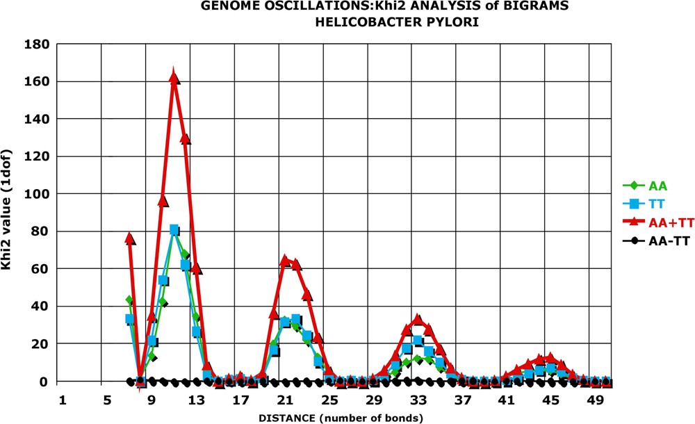
KHI2 analysis of significance of genome oscillations (AA; TT): Helicobacter pylori. Statistical significance of the difference between the observed and expected number of occurrences of bigrams. The ‘raw’ data of the Helicobacter genome (see Fig. 1) were normalised and ‘pruned’ as in Table 3. The resulting values for the bigrams AA, TT, their sum (AA + TT) and their difference (AA − TT) were analysed by Khi2 statistics: and the results plotted as a function of d. For each value, there is one degree of freedom. It is apparent that Khi2 values are very great for distances (11, 21, 33, 44) corresponding to the oscillation peaks (compare with Fig. 2) and the probability that they are due to chance is smaller than 10−40. Importantly, the significance of the sum of is huge, while that of the difference is 0. This proves that oscillations of and vary in phase, are of equal importance and should be added in order to estimate the overall oscillations.
All genomes display the oscillations. However, the amplitude of oscillations may be quite different from species to species. A series of figures (Figs. 2–4 and Figs. A6–A12) illustrates this fact. Two of the displayed genomes have strong oscillations, two have very weak ones, and in Figs. A11 and A12 an average procaryotic genome presents, as expected, intermediary amplitudes. It is important to stress that even one of the weakest genomes, Caulobacter crescentus, has statistically significant oscillation amplitude: the probability that its is due to chance is 10−18 for 1 GUS and of course much smaller for its true genome size. A series of figures (Fig. 5 and Figs. A13–A16) partially answers the question: “Which is the best discriminator for the differences in amplitude of oscillations between different species?” There are 16 kinds of bigrams and ways of combining all of them in a single descriptor. I have proceeded step by step by the Khi2 approach mentioned before. The AA, TT, GG and CC bigrams vary always in phase in all the 80 genomes analysed. Their sum (AA + TT + GG + CC) constitutes a good general descriptor and interspecies discriminator. It will be referred to as the combination I of bigrams. The sum of AC, CA, GT, TG, AT and TA always varies in the opposite phase to the combination I and the values lead to a better discrimination between different species than combination I. It will be referred to as the combination II. In a few interspecies comparisons, the combination III leads to more pronounced differences between genomes than combinations I or II. The and bigrams lead frequently to ambiguous results and I did not use them in a systematic manner. In consequence, the calculations are done routinely with combinations I, II and III, and the average values from the three combinations are shown. One can see in Figs. 6 and 7 that the three combinations give very similar results both for species with great oscillation amplitude (‘high’ genomes) and for species with small amplitude of oscillations (‘low’ genomes). Four examples of ‘high’ genomes are given in Fig. A17 and four examples of ‘low’ genomes in Fig. A18.
Genome oscillations: three combinations of bigrams: Helicobacter pylori. There are 215 possible combinations of grouping the 16 kinds of bigrams: AA+AT+TA+⋯+TG, AA−AT+TA+⋯+TG, AA−AT−TA+⋯+TG, etc. All have been explored by the approach described in Fig. 5 (i.e. if the addition increases the significance, then it is kept and if it decreases, it is not kept). Finally, three best combinations were retrieved (designated I, II and III). In all genomes, II gives more pronounced oscillations than I, and in the majority of genomes, II is better than III. Numbers of bigrams correspond to the ‘pruned’ values: , with .
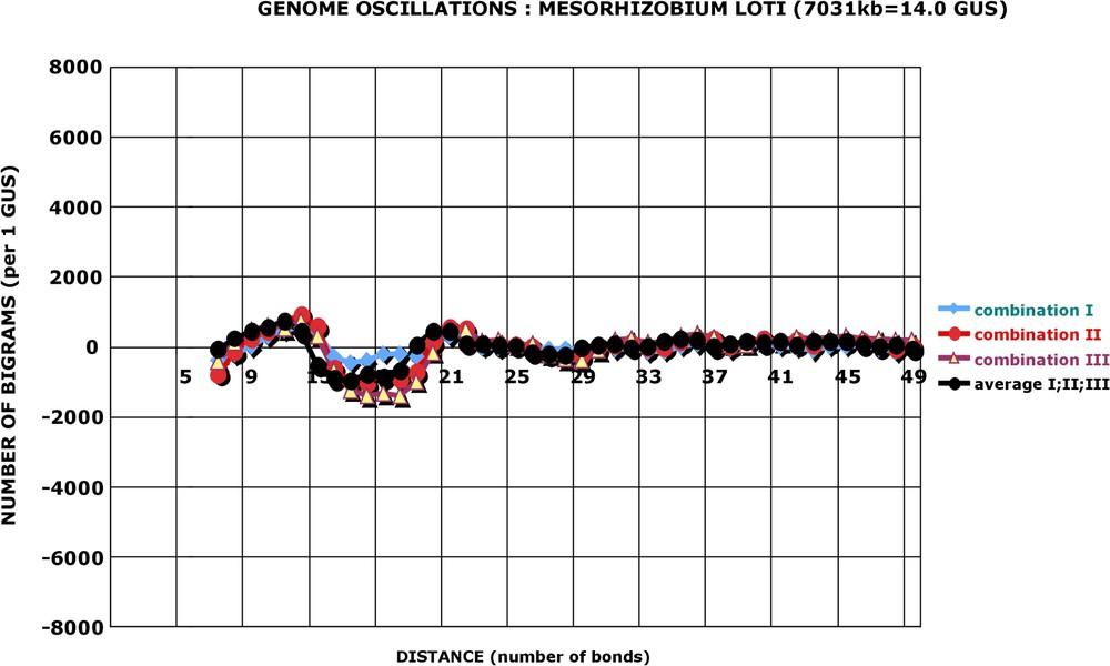
Genome oscillations: three combinations of bigrams: Mesorhizobium loti. The oscillation amplitude of Mesorhizobium is much smaller than that of Helicobacter, but it is still discernable (calculation as in Fig. 6).
The next series of data pertains to the phylogenetic and taxonomic relations between various species and their genomic oscillations. It is not surprising that genomes allocated to the same family display almost identical patterns of oscillations. Two species of Vibrionales (Fig. A19) on the one hand, and two species of Rickettsiales (Fig. A20) on the other hand, illustrate this notion. Notice that there is a small but conspicuous difference between the two families: although the second peak is in both cases at , the first peak is closer to in Vibrionales and closer to in Rickettsiales. Figs. A21 and A22 give examples of different patterns of oscillations for species classified in the same family. This again is not surprising, because of the well-known difficulties in the taxonomy of procaryotes. On the contrary, the results shown in Fig. 8 are completely unexpected. Two species belonging to two different kingdoms, Methanopyrus from Archae and Aquifex from Bacteria display practically identical genome oscillations. The same is true for the second pair of species, Methanosarcina from Archae and Coxiella from Bacteria (Fig. 9). However, and it seems to me very important, the genomic oscillations of the first pair of species are significantly different from those of the second pair; the first pair is ‘high’ in oscillation amplitude, while the second is ‘low’. Furthermore, their general patterns appear quite different (compare Figs. 8 and 9). Thus, during the one or two billion years, which have separated the Archae lineage from the Bacterial one, evolution has selected both specific and similar overall properties of genomic sequences. It is clear to me that the classification and the comparative studies of genomic oscillations, taking advantage of various classical techniques like principal component analyses, distance matrices (etc.), will shed a new light on the phylogeny, taxonomy and classification of procaryotes.
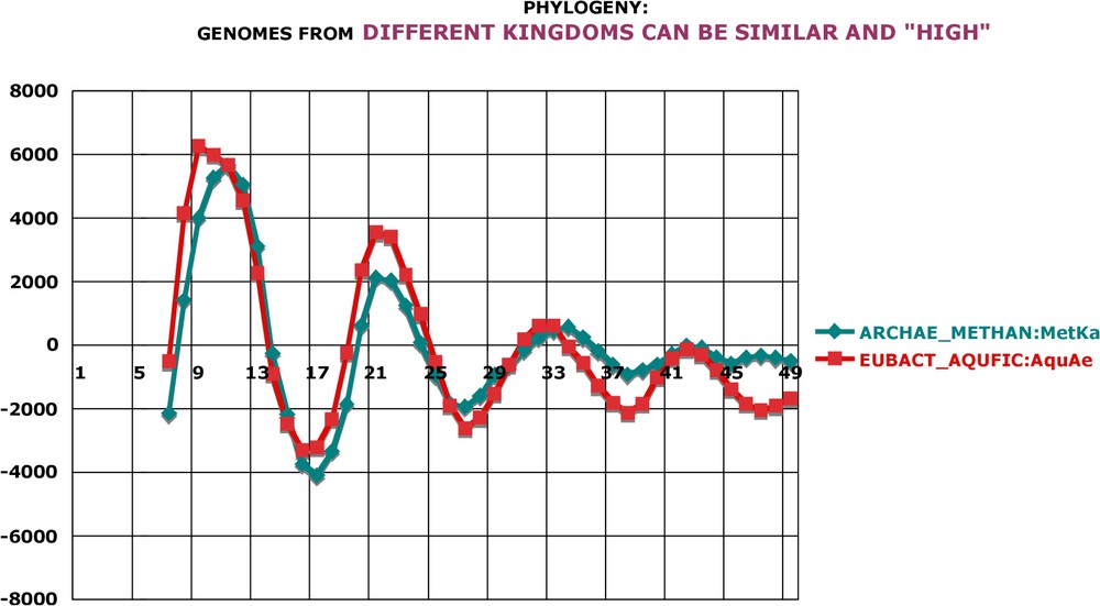
Phylogeny: genomes from different kingdoms can be similar and ‘high’. Methanopyrus and Aquifex are allocated to different kingdoms (Archaea and Bacteria). Interestingly, their genome oscillations are quite similar in amplitude, which is high. Calculation as in Fig. A17.
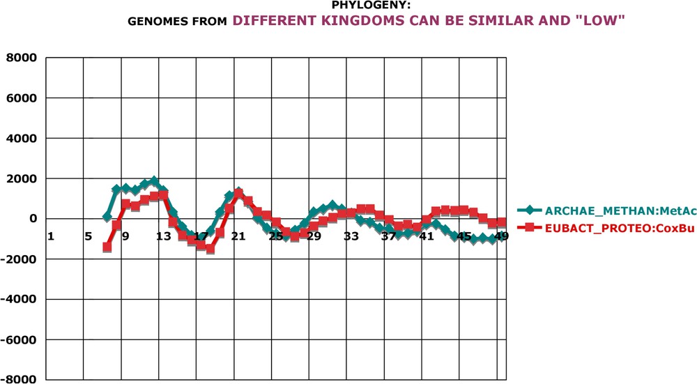
Phylogeny: genomes from different kingdoms can be similar and ‘low’. Methanosarcina is an Archaeon and Coxiella is a Bacterium. However, their genome oscillations are very similar, both in amplitude and in general pattern. Notice that the amplitude of these two genomes is about four times smaller than that of the preceding pair of species shown in Fig. 8. Calculation as in Fig. A17.
There is no relation between the size of a genome and the amplitude of its periodic oscillations. Fig. A23 shows an example where a ‘big’ genome has a high amplitude and a ‘small’ genome has a low amplitude (Thermoanaerobacter versus Ureoplasma). The contrary is shown in Fig. A24, where a ‘small’ genome, Phytoplasma, has high oscillations, while a ‘big’ genome, Escherichia, has low oscillations.
There is no correlation between the overall (G + C) content of a genome and its periodic oscillations. In Fig. 10, two species displaying the same (G + C) content (close to 51%) present very different oscillations. In Fig. 11, the genome oscillation index, which estimates the overall extent of oscillations (see legend), is plotted as a function of (G + C). Although one finds a cluster of (G + C) rich genomes, which are ‘low’, there is no obvious correlation when all 80 genomes are examined.
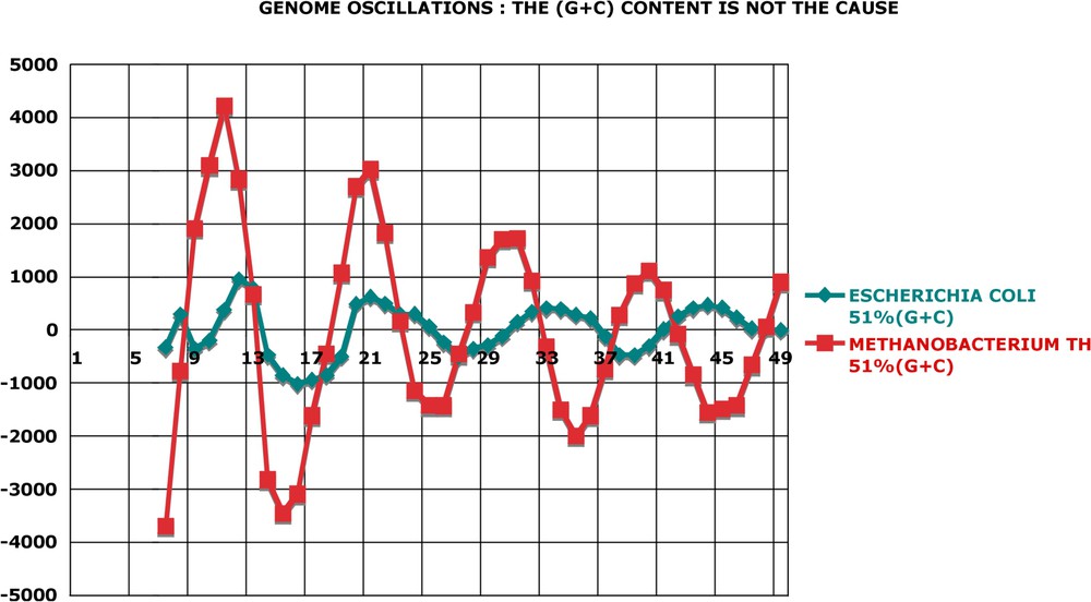
Genome oscillations: the (G + C) content is not the cause. Methanobacterium and Escherichia have practically the same (G + C) content of their genomes. This suggests that this property is not the cause of conspicuous differences in the amplitude of their oscillations. This conjecture is proven by the scatter plot of Fig. 11. Calculation as in Fig. A17.
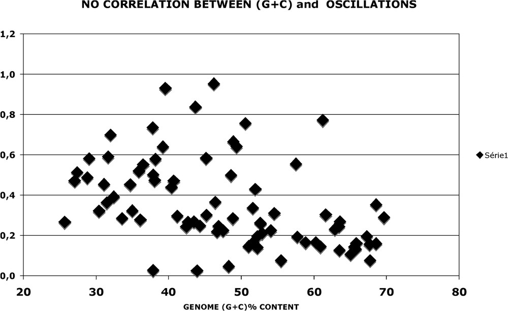
No correlation between (G + C) and oscillations. Oscillations of each genome (1 GUS) were calculated as in Fig. A17. The oscillation index is a measure of the amplitude equal to the sum of for (9+10+11+12+20+21+22+30+31+32+33+42+43, i.e. peaks) minus the sum of for (7+15+16+17+25+26+27+36+37+46+47+48, i.e. valleys). It is normalised to 1 for the corresponding values of the nucleotide sequence of genes coding for alpha helical proteins (1 GUS, see Fig. 13). In this manner, the index of Helicobacter pylori genome, the highest one, is 0.93. The scatter plot shows that there is no correlation between the (G + C) content of the genome and its oscillations.
Last points deal with the main question, the cause of periodic oscillations of genomic sequences. The average estimation of the period length is 11 phosphodiester bonds (based upon measurements of 80 genomes). The overall pattern can be easily fitted to an exponentially dampened sinusoid with this periodicity. This suggests, but does not prove, that the two sinusoids, the genomic sinusoid (this work) and the proteomic sinusoid [3] have the same cause, since the periodicity of 11 nucleotides found here is equivalent to the periodicity of 3.5 amino acids observed previously [3] (3.5 codons ∼11 nucleotides). This is a striking and certainly non-coincidental correspondence to one turn of the alpha helix in proteins. However, periodicities of 10–11 base pairs per turn have been generally interpreted as resulting from physicochemical constraints of DNA or chromatin (see [3] for a review). I have approached this dilemma in two ways.
First, I have calculated the frequencies of bigrams in the protein coding sequences of Open Reading Frames retrieved from the TIGR data base. The periodic oscillations are practically identical, both in amplitude and in position, for the complete genomes and for the collections of corresponding ORFs. Now, in the collections of ORFs, the non-coding intergenic sequences are absent. Depending on the species analysed, these non-coding sequences represent 10 to 30% of the total length. If these intergenic sequences had significant effect on the periodic oscillations in the genomic sequences, this would be easily detected. However, when the genomic and proteomic periodic oscillations of nucleotides are compared, the regression is practically equal to 1.0 with very little scatter (see Fig. 12). This suggests that non-coding sequences do not contribute to the amplitude of oscillations. Alternatively, one could argue that the non-coding sequences have the same properties as the protein-coding ones.
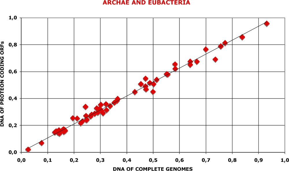
Nucleotide oscillations are in the protein coding sequences of genomes. On the one hand, the index of nucleotide oscillations was calculated for the whole genomes as in Fig. 11. On the other hand, for each species, the complete set of nucleotide sequences coding for proteins was retrieved from the CMR data base, the values were calculated (as in Fig. A17) separately for each ORF, then summed up and the index calculated as above. The regression coefficient is 0.98 and the correlation coefficient 0.99 for the two datasets.
The second approach is more telling. I have retrieved (see Section 2 for details), from the protein structure data base (PDB) and from EBI, the nucleotide sequences of genes or gene segments coding for proteins which have been crystallized and whose 3D structures have been determined directly by X-ray diffraction (in a very few cases, this was done by NMR). Table A1 gives the accession numbers of the structure determinations. I have made two sets of data. The first contains 86 genes coding for proteins that are rich in alpha-helical segments and have no β structures. The average of alpha-helix content of these ‘alpha genes’ is 59% and their total length is 51 423 nucleotides. The second set is composed of 30 genes, which code for proteins practically devoid of alpha-helix but rich in β (51%) and other non-helical structures. They constitute the ‘non-alpha genes’ (23 753 nucleotides in total). I am aware that these are small figures, both in the number of genes and in the number of nucleotides. But ‘pure alpha’ or ‘pure non alpha’ proteins are quite scarce in the PDB and I have tried not to collect duplicate sequences. Obviously, these two sets of genes are not representative of the diversity of proteins, since most of them are from vertebrates and not from procaryotes. I have performed the expectancy-rectified analysis of bigrams on these two sets of genes, in exactly the same way as on the whole genomes. The question is: do the ‘alpha genes’ or ‘non-alpha genes’ show the periodic oscillations of nucleotides? Fig. 13 shows that the ‘alpha genes’ have periodic oscillations at the same positions and of a similar amplitude as the ‘high’ genomes like Helicobacter or Aquifex. There are not enough sequences of ‘alpha genes’ in the data bases to constitute 1-GUS length. Therefore, the bigrams are normalized to 0.1 GUS in Fig. 13 and the amplitudes have to be multiplied by 10 to be compared to Fig. 6 and Fig. A17. The Khi2 analysis (Fig. A25) shows that, in spite of the small number of nucleotides analysed (ca. 0.1 GUS), the maximal positive oscillations at and are highly significant: the probability of their occurrence by chance is close to 10−3 and 10−4, respectively (Fig. A26). For the occurrence of both of them, the expectancy is 10−6. On the contrary, the ‘non-alpha genes’ are devoid of oscillations (Fig. A27). All their apparent deviation from randomness has a more than 10% probability to occur by chance. I believe that this demonstrates that the periodic oscillations of bigrams are correlated with the coding capacity of DNA for alpha-helical proteins. However, a correlation does not establish the causality.
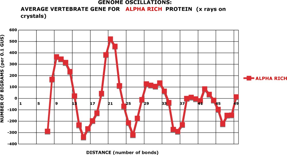
Nucleotide oscillations of an average gene coding for alpha helical proteins. Proteins (see the ID in Table A1) rich in alpha helices and devoid of beta sheets were retrieved from EBI and the nucleotide sequence oscillations calculated in the same manner as for the ORFs of a genome (see Fig. 12). Since the total length is much smaller than even the smallest genome (there are only 86 genes!), the ordinates are normalised to 0.1 GUS instead of 1 GUS. The four peaks and valleys are present like in genomes.
The final set of data constitutes, in my opinion, the most interesting series of results. I have retrieved from the TIGR CMR Data Base all pairs of genes coding for pairs of homologous proteins ensuring the same biochemical function – as attested by the expert (TIGR) annotation, as well as by the members of consortia who sequenced the DNA (original annotation). I have used a very stringent criterion for establishing homology: a P value smaller than 10−20 (for the majority of protein pairs, the P value is in fact much smaller than 10−20, see Table A2). I have selected by the ‘best-hit’ approach only orthologous pairs and have eliminated paralogous genes. In this way, I have compared five ‘high’ genomes (Aquifex = AquAe, Helicobacter = HelPy, Methanococcus = MetJa, Methanopyrus = MetKa and Wollinella = WolSu) with five ‘low’ genomes (Bdellovibrio = BdeBa, Mesorhizobium = MesLo, Mycobacterium = MycLe, Pirellula = Pire1 and Rhodopseudomonas = RhoPa) in all pairwise combinations of species. Each pair of species compared provides several hundred pairs of homologous genes for further analyses. This constitutes therefore a robust set of several hundreds of thousands of nucleotides. Table A2 gives an example of the beginning of a list of pairs of genes in the comparison, Helicobacter versus Mesorhizobium.
It is obvious, but nevertheless important, to stress that the homologues between a pair of species, say XY, can be quite different from those of the pair of species XZ or YZ (the complete list of homologues can be consulted in the supplementary material). Thus, in addition to the ubiquitous homologues, which are present in all genomes (e.g., the genes coding for the threonyl–tRNA synthetase), hundreds of different homologues are specific for the pair of species considered and depend, of course, on the phylogenetic relationships between species. A second remark is as important (and as obvious) as the first. Pairs of homologous proteins display significant identity/similarity of their amino acid sequences (it is the very basis for considering them as homologues), but, at the same time, an important fraction of their sequences is different (e.g., in proteins HP0033 and mll0663, 56% of their sequences are different, in spite of a P value of 10−146 (Table A2). Having these considerations in mind, we can analyse the results of the comparisons.
In Fig. 14 and Figs. A28–A32, one can see that genes from a ‘low’ genome, coding for the same function as their homologues from a ‘high’ genome, display nucleotide-sequence oscillations of small amplitude. The genes from a ‘high’ genome, homologous to those from a ‘low’ genome, always have a large amplitude of oscillations. There is no exception to this rule in all the pairwise combinations of species. Only one example is given for Helicobacter, all five comparisons analysed are given for Aquifex, and the remaining comparisons can be consulted in the supplementary material. In agreement with this rule, the comparison of homologues from ‘high’ genomes with different ‘high’ genomes leads to large oscillation amplitudes, and ‘low’ with ‘low’ to small oscillation amplitudes.
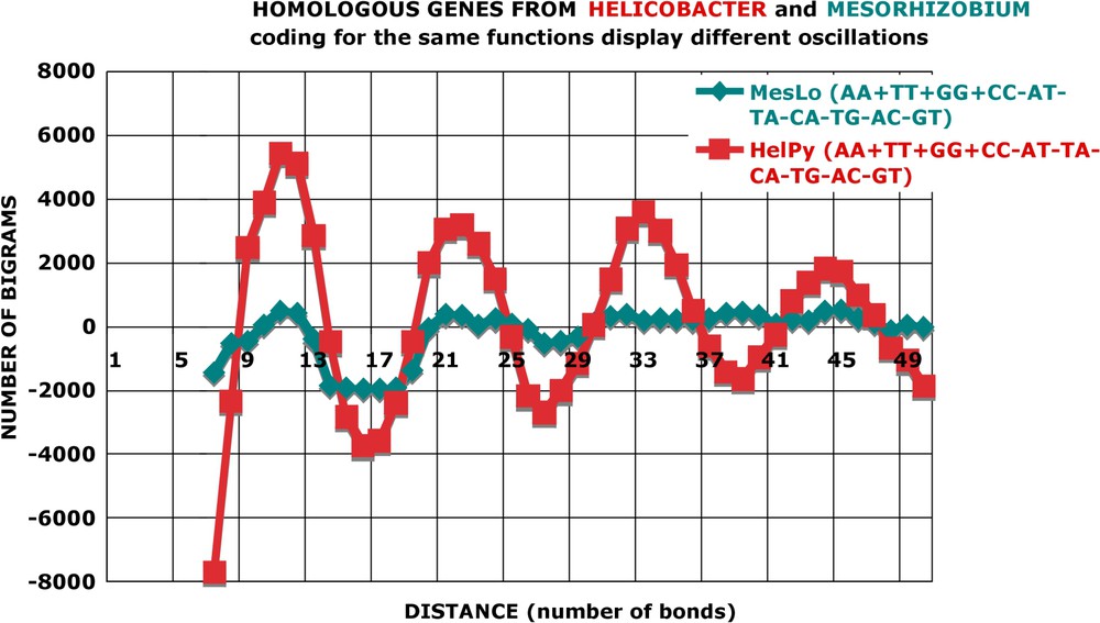
Homologous genes from Helicobacter and Mesorhizobium coding for the same functions display different oscillations. Pairs of homologous proteins from Helicobacter and Mesorhizobium were retrieved from TIGR-CMR with a stringent homology criterion: P value smaller than 10−20; only pairs of orthologous genes were kept (the ‘best-hit’ approach), while paralogous genes were eliminated. According to the annotation of the data base, the members of a pair have presumably the same function in the two species. For each set of 434 orthologous genes (see Table A2 for the complete list), the nucleotide oscillations were calculated as for the genomic ORFs (see Fig. 12) and the values shown: homologous genes from two species have different oscillation amplitudes. Notice that the homologues of HelPy to MesLo have the same oscillations as all the genes from HelPy and, reciprocally, the homologues of MesLo to HelPy have the same oscillations as all the genes from MesLo, although they represent only a small fraction (434/7887=6%) of total genes (compare Fig. 14 with Figs. 3 and 4). Thus, the genomic style of proteins is an intrinsic and specific characteristic of a species.
Without the results of the comparisons illustrated in Fig. 14 and Figs. A28–A29, one could argue that large oscillations observed in Helicobacter or Aquifex were due to a fraction of their genes having some special properties, such as unusual codon bias, specific location on the chromosome, some unknown and exceptional function, or any kind of a hypothetical intra-genome heterogeneity. These types of genes would be absent or scarce in ‘low’ genomes.
However, the results of these comparisons of homologues refute such hypotheses, because the genes coding for the same function, located in all different and not homologous section of genomes (there is no synteny between various ‘high’–‘high’ or ‘low’–‘low’ genomes), can be either ‘high’ or ‘low’, depending on their origin. These results demonstrate, I believe, that the oscillation amplitude is an intrinsic and general property of a genome. Obviously, this idea is not at all in contradiction with the notion that, within a ‘high’ genome, some individual genes would have large oscillations and others very small ones, with all possible intermediates from ‘high’ to ‘low’. It simply states that a gene from a ‘high’ genome would have a more pronounced amplitude of oscillation than its homologue from a ‘low’ genome. It should be borne in mind that this concept cannot be tested directly on single genes because of insufficient statistics. To obtain statistically significant data, one has to analyse a sequence of at least 10 000 nucleotides. There are practically no protein coding genes of that length in procaryotes.
Taken at face value, the two main findings of this investigation can be summarized quite simply: (i) alpha-genes have high nucleotide oscillations while non-alpha genes have no oscillations; (ii) genes present in ‘high’ genomes have high nucleotide oscillations, while their homologues coding for the same function but occurring in ‘low’ genomes have very weak nucleotide oscillations.
The most straightforward conclusion (but is it a true syllogism or a specious argument?) would be that homologous proteins coding for the same function would be richer in alpha-helical segments when derived from organisms with ‘high’ genomes, and significantly poorer in alpha-helical segments when derived from organisms with ‘low’ genomes. Such an idea is certainly a heterodox one. It can be easily refuted by crystallizing and determining ab initio the 3D structure of a series of homologous proteins from, say, Helicobacter and Mesorhizobium. However, I am not sure that there are many grant awarding agencies that would be willing to sponsor the investigation of such heterodox ideas, although the aim of the structural genomics is precisely to tackle problems of relations between protein structures and genomes.
A much easier approach is to investigate the relations between proteins from ‘high’ and ‘low’ genomes by the various secondary structure prediction methods, with their well-known limitations and uncertainties. Preliminary results are encouraging and will be presented elsewhere (Slonimski, in preparation).
One could also envisage an alternative explanation for the observed differences between the homologous genes from ‘high’ and ‘low’ genomes: homologous proteins would have the same degree of alpha helicity in both cases, and the striking differences in the periodic oscillations of nucleotide sequences would result from different ways of constructing alpha helices in ‘high’ and in ‘low’ organisms. By different ways of constructing alpha helices, I can imagine, for instance, a systematic usage of a specific subset of amino acids or codons, which will be common to all proteins in a ‘high’ species, and systematically different from it in a ‘low’ species. Such an interpretation is in line with the concept of the genomic style of proteins [7]. This is under study.
The last question concerns membrane proteins. It is well known that the true membrane proteins consist of one or more transmembrane alpha-helices, with helix axes normal, or close to normal, to the plane of the bilayer. Goffeau et al. [9] have estimated that some 30% of the genome of Saccharomyces cerevisiae codes for membrane spanning proteins. It is generally admitted that similar values are also true for procaryotes. However, very few membrane proteins have been crystallised and X-rayed, and as far as I know, not a single one from the species that display major differences in the amplitudes of genomic oscillations. This is a major issue, especially in view of the fact that the span of oscillations described here is similar to the length of the transmembrane spans (nucleotide bonds up to 51; polypeptide bonds).
Two extreme interpretations can be proposed: (i) ‘high’-oscillation genomes have more membrane spanning proteins, and/or more membrane spanning segments within homologous proteins, than ‘low’ genomes; (ii) ‘high’ genomes construct their membrane spans with a set of codons and amino acids very different from the set used by ‘low’ genomes.
Whatever the answers to the questions raised by the discovery of nucleotide sequence oscillations (in biology, the answers to radical questions are, alas, more often intermediate than extreme), further studies of this unexpected property of genomes should shed, I believe, a new light on some major problems of genomics.
Acknowledgements
I would like to thank, first of all, my son-in-law, Joël Prince ‘développeur 4e dimension’ (joelprince@free.fr), for writing a programme for my personal computer, Dr. J. Radomski (janr@icm.edu.pl) from the University of Warsaw, for numerous discussions in the last few years, and Dr. C.J. Herbert from CGM, for looking over the English. Drs. S. Blanquet, É. Brezin, A. Danchin, P. Joliot and V. Luzatti are thanked for stimulating criticisms and comments during the ‘Conférence-débat sur la génomique analytique et comparative’, which I have organised at the French Academy of Sciences, on 7 February 2006 and where I have presented this contribution. PPS is Professor Emeritus (active) of University Paris-6.
1 Figs. A1–A29 and Tables A1–A2 can be found in the web-available supplementary material.