

1 Introduction
The modelling of commercial exploitations of renewable biological resources is a challenging task, as it includes the non-linear interaction of biological, economic and social components. In recent past years, many researchers have paid attention to the management of renewable resources, considering different parameters and externalities. In the management of common property renewable resources (such as fisheries, forestry and wildlife) harvested by competing individuals, societies or countries, the problem known as “The tragedy of commons” after Hardin [1]. Later on Clark [2], Masterton-Gibbons [3], Conrad [4] discussed many issues and techniques on this subject. Clark [2] discussed the problem of non-selective harvesting of two ecologically independent populations obeying logistic growth. Kar and Chaudhuri [5] discussed non-selective harvesting of a multispecies fishery. There are also some papers on competitive fish-species and on prey-predator models (see Gordon [6]; Datta and Mirman [7]; Bischi and Kopel [8]; Dubey et al. [9]; Bischi et al. [10]). Most of the prey-predator models consider a single prey called the focal prey; however, many authors have emphasized that the presence of alternative foods can effect biological control through a variety of mechanisms. For example, the presence of one prey species can have negative effects on the population of another prey species, by allowing the population of a shared predator to increase, thus leading to higher predation rates upon both prey items. In contrast, alternative prey can also lower predation on focal prey because of predator preference for alternative prey resources (Abram and Matsuda [11]). In such instances, the alternative prey can have a positive effect on population densities of the focal prey. Many massive piscivores, including spiny dogfish in the North-West Atlantic, and Pacific hake, undertake extensive seasonal migrations on a spatial scale much larger than the habitat occupied by some of their prey, and the development of realistic models for these prey-predator systems will require consideration of alternative prey. Vence [12], Spencer and Collie [13] have considered alternative prey in their models.
Methods used for managing predators, and associated public perception, are a crucial consideration in developing effective systems of management for predators and prey. Controlling predator populations to reduce predation on a threatened or endangered species may be difficult to achieve. Keeping wolf and cougar (wild American cat) populations in check might require reducing alternate prey. Control of mule deer populations in Sierra mountains of California might be required in addition to reductions in cougar numbers to prevent extirpation (complete destruction) of Sierra Nevada big horned sheep populations. The Alberta Government has issued additional hunting permits for moose and deer in an attempt to reduce alternate prey for wolves, hoping to reduce wolf numbers and thereby predation pressure on caribou.
In this study, we develop a simple, two species predator-prey model that incorporates the effect of alternative prey. We consider logistic production function of prey and a Holling type-II predator functional response (Holling [14]) so that there may present multiple equilibrium population levels. In our model, the growth rate of prey is formulated as
| (1) |
The growth rate of predator population is taken as
| (2) |
Here, as the focal prey population (N) increases, the predator uses less alternative prey and when N → K the mass of alternative prey consumed tends to zero, and conversely, as the focal prey decreases, the predators increase their feeding on alternative prey. If N → 0 then dP/dT → (d1 − γ1)P. Thus even in case of the extinction of the focal prey the predator population maintains its growth rate, varying linearly with its density.
Now we introduce dimensionless variables by the following substitutionN = ax, P = ray/α1, T = t/rthen our Eqs. (1) and (2) become
| (3) |
| (4) |
Lettingwe can write the governing equations as
| (5) |
| (6) |
For considering the exploited prey-predator system, we introduce scaled harvesting efforts E1 and E2 for prey and predator, respectively and then the equations governing our model become
| (7) |
| (8) |
The Note is organized as follows. The existence of different equilibrium points are considered in section 2. Stability analysis and bifurcations are given in section 3. In section 4, detailed numerical simulations are given. The Note ends with a conclusion in section 5.
2 Equilibrium of the model
Lettingandϕ3(x) = βϕ1(x) + d(1 − x/η) − (E2 + γ)the governing equations (7) and (8) become
| (9) |
| (10) |
The prey zero growth lines are obtained by setting dx/dt = 0, which gives ϕ1(x) = 0, y = ϕ2(x) that is x = 0 (y-axis) and the curve y = ϕ2(x). The curve y = ϕ2(x) passes through the points (0, 1 – E1) and (η(1 − E1), 0).
We see that
Thus, , andϕ2′(η(1 − E1)) = − (1 − E1 + 1/η)
Thus if η(1 − E1) > 1, then and are of opposite signs and so ϕ2(x) has a local maximum between x = 0 and x = η(1 − E1). The predator zero growth lines are obtained by setting dy/dt = 0 i.e. y = 0 (x-axis) and ϕ3(x) = 0. Thus isoclines of predator other than x-axis are the zeros of ϕ3(x).
These are given by
| (11) |
| (12) |
Here we investigate the different cases for positive zeros of ϕ3(x) to have interior equilibrium. From the above discussion we already have two boundary equilibria P0(0, 0), P1((1 − E1)η, 0) while P1 exists if E1 < 1.
Case 1.
If and E2 + γ − d < 0, that is, if , then ϕ3(x) has only one positive zero given by
| (13) |
Thus, in this case, the trivial equilibrium P0(0, 0) always exists, the boundary equilibrium P1((1 − E1)η, 0) exists if E1 < 1 and the only interior equilibrium P2(x2, ϕ2(x2)) exists if E1 < 1 − x2/η and .
Here it can be observed that if P2 exists then P1 also exists.
Case 2.
Let , E2 + γ − d < 0. In this case only one positive interior equilibrium may be obtained if (d − γ) > 0, (β − d/η) < 0 i.e. if d > max{γ, βη} and .
In this case x = x2 is a positive zero of ϕ3(x) and P2(x2, ϕ2(x2)) is a positive interior equilibrium while E1 < 1 − x2/η along with the above conditions. Therefore, in this case, the trivial equilibrium P0(0, 0) always exists, the boundary equilibrium P1((1 − E1)η, 0) exists if E1 < 1 and the interior equilibrium P2(x2, ϕ2(x2)) exists if E1 < 1 − x2/η, d > max{γ, βη} and . Here also we see that the conditions of existence of P2 suffice the existence of P1.
Case 3.
Let
More explicitly,
Then there are two positive zeros of ϕ3(x) which are x1, x2 given in (12) and
It is observed that at P2 & P3 both the species co-exist under some conditions stated above.
3 Stability analysis
The Jacobian matrix for our model is
| (14) |
Since therefore and from the expressions of ϕ2(x), ϕ3(x) we get
We first investigate the stability at the trivial equilibrium P0(0, 0), the boundary equilibrium P1((1 − E1)η, 0), and then the discussion of stability of interior equilibrium will be considered in different cases as they appear in terms of their existence.
At P0(0, 0) the corresponding community matrix is simplified to be
| (15) |
At P1((1 − E1)η, 0) the matrix J is evaluated as
| (16) |
Now we go through the following cases for discussing the stability at interior equilibrium, taking the references of the cases of existence of equilibrium points discussed earlier.
Case 1.
Letthen only the positive interior equilibrium is P2(x2, ϕ2(x2)). At this equilibrium
The characteristic equation is
| (17) |
Since x1, x2 are the roots of ϕ3(x) = 0, therefore from Eq. (11) we have
Thus ϕ1(x2)ϕ2(x2)ϕ3′(x2) < 0 as ϕ1(x2), ϕ2(x2) are positive and hence (17) has one positive and one negative root. Therefore in this case P2(x2, ϕ2(x2)) is an unstable equilibrium.
Case 2.
Let
In this case P2(x2, ϕ2(x2)) is the only positive interior equilibrium. As in Case 1, and the equilibrium is unstable at P2(x2, ϕ2(x2)).
Case 3.
Let
In this case two interior equilibrium points P2(x1, ϕ2(x1)) and P3(x2, ϕ2(x2)) exist.
Now we investigate the stability at P2 and P3.
At P2(x1, ϕ2(x1)) the community matrix is reduced to
| (18) |
| (19) |
Now are all positive under the conditions of existence of P2(x1, ϕ2(x1)). Thus by Descartes’ rule of signs, P2 is a node or a focus or a centre. By Routh-Hurwitz condition, the equilibrium at P2(x1, ϕ2(x1)) is stable if , and is unstable if . A limit cycle is expected closed to the curve . Now implies that or
Or,
| (20) |
| (21) |
Thus if i.e. if E1 > ϕ(E2) then P2(x1, ϕ2(x1)) is locally asymptotically stable and if E1 < ϕ(E2) then P2(x1, ϕ2(x1)) is unstable in the positive quadrant of x1x2 − plane. For E1 = ϕ(E2) i.e., for the roots of (19) ur discussion on stability at P3(x2, ϕ2(x2)) we see that the characteristic equation of the community matrix at P3 is
| (22) |
Since we have earlier discussed that for the existence of P3; therefore by Descartes’ rule of signs, the roots of (22) are both real and of opposite sign. Thus P3(x2, ϕ2(x2)) is an unstable saddle point whatever the sign of may be.
We now state the following theorem: If the conditions (H1), (H2) and (H3) are satisfied then: (i) P0(0, 0) is stable if E1 > 1, E2 > d − γ. (ii) P1((1 − E1)η, 0) is stable if and is unstable when (iii) P2(x1, ϕ2(x1)) is stable if E1 > ϕ(E2) and is unstable when E1 < ϕ(E2). (iv) P3(x2, ϕ2(x2)) is always unstable. We notice thatTheorem 1
Hence by the Hopf bifurcation theorem (Hassard et al. [15]) the system (9) and (10) enters into a Hopf type small amplitude periodic oscillation at the parametric values E1 = ϕ(E2) near the positive interior equilibrium P2(x1, ϕ2(x1)). Hence we may state the following theorem: For E1 = ϕ(E2) a super critical Hopf bifurcation takes place for the equilibrium P2. Let us consider the Jacobian matrix (18). By direct calculation the eigen values are given by:Theorem 2
Proof
Or, , where T = trace of J and D = det J.
Now for T = 0, D > 0 and in corresponding to the values of E1 = ϕ(E2) the matrix has two purely imaginary eigenvalues . Moreover . Thus, all conditions of Hopf theorem are satisfied and a stable limit cycle for E1 < ϕ(E2) may be found. All these conditions together prove the existence of a super critical Hopf bifurcation for the equilibrium P2.
We also have the following result on global stability in the region of local stability:
Theorem 3
If P2(x1*, ϕ2(x1*)) is locally asymptotically stable, then it is globally stable in the interior of R2+.
Proof
If possible, let there be a periodic orbit Γ = (x(t), y(t)), 0 ≤ t ≤ T with the enclosed region Ω and consider the variational matrix J about the periodic orbit,
We compute
For biological equilibrium in the region of local stability it can easily be seen that
Therefore, Δ < 0 and the periodic orbit Γ is orbitally asymptotically stable (Cheng et al. [16] and Hale [17]). Since every periodic orbit is orbitally stable then there is a unique limit cycle. From the Poincare–Bendixson Theorem, it is impossible to have unique stable limit cycle enclose a stable equilibrium. This is the desired contradiction. Hence there is no limit cycle and P2 is globally stable.
As the analytical results already indicate, the existence and stability of the interior equilibrium, as well as the stability of the trivial and boundary equilibrium will depend on the specific parameters that determine the dynamic evolution of the resource stock and the population. In the next section we present a more in-depth analysis of the complexity of the long run dynamics of population and resource stocks as they depend on the parameters of the system. The results are obtained through a detailed numerical and global bifurcation analysis.
4 Numerical simulations
We consider numerical simulations of different cases to understand the theoretical findings.
For η = 60, β = 4, d = 0.6, γ = 0.9 we have the bifurcation diagram shown in Fig. 1, and the point (E1, E2) = (0.9, 2.69) marked by * is in stable region and the point (E1, E2) = (0.75, 2.69) marked by • is in the region of unstability.
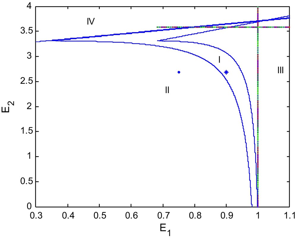
Bifurcation diagram in the (E1, E2) plane.
Fig. 1 illustrates a detailed picture of the possible long run dynamics as they depend on the values of the harvesting efforts E1 and E2 for the benchmark case. The various dynamic behaviors are described in separate figures that show the corresponding stable and unstable equilibria in phase space together with selected time paths.
In brief, the bifurcation diagram as presented in Fig. 1 allows us to investigate the specific combination of efforts E1 and E2 that may cause the model to shift from sustainable long run equilibrium towards a limit cycle and finally the collapse of the system. Local bifurcation theory is the numerical tool that determines the boundaries between these regions in parameter space (Fig. 2).
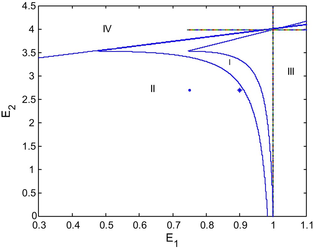
Bifurcation diagram for d = 0.9.
We see that as d increases from 0.6 to 0.9 the area of region of stability decreases as shown in Fig. 2. If we increase d again to 1.0 the stable region of stability shrinks more, as depicted in the Fig. 3.
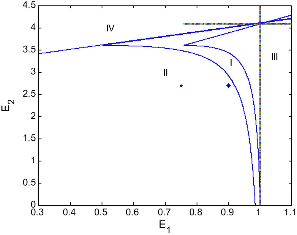
Bifurcation diagram for d = 1.0.
Figs. 1, 2 and 3 show bifurcation diagrams in the (E1, E2)-plane for d = 0.6, 0.9 and 1, respectively. We see that the stability region becomes smaller as d becomes larger. We may say that d destabilizes the coexisting equilibrium P2. Thus for the long run sustainability of a prey-predator system, this might require reducing alternative prey (Fig. 4).
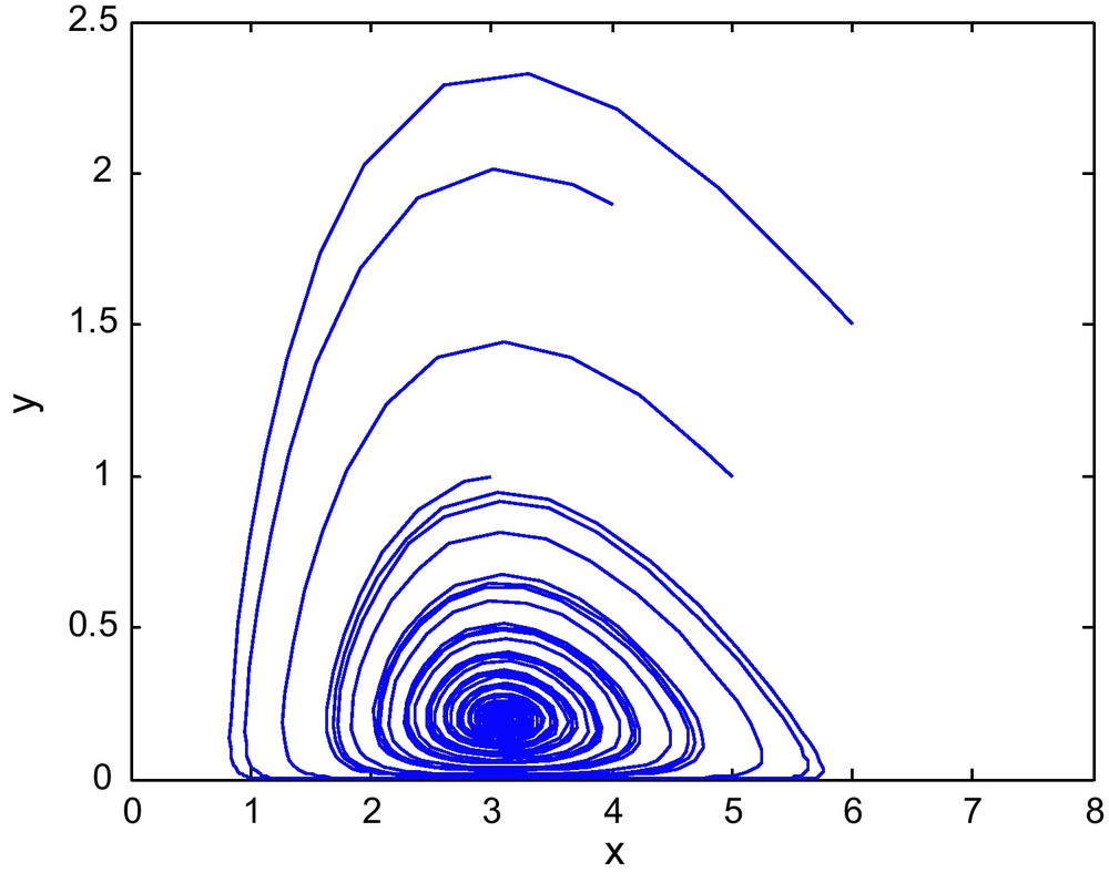
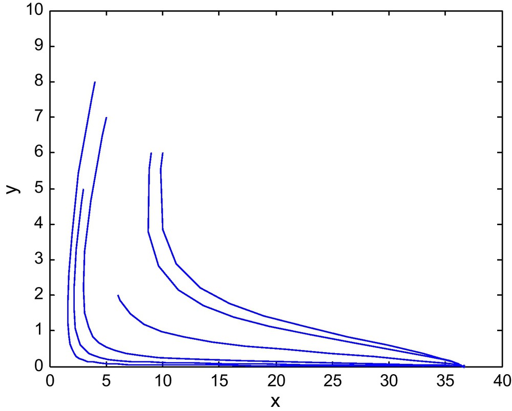
The phase diagram for (E1, E2) = (0.9, 2.69) with d = 0.6.
The phase diagram for d = 0.06 is shown in Fig. 4. When d increases to 0.9 or 1.0 then the point (E1, E2) = (0.9,2.69) marked by * lies outside the stable region and the interior equilibrium becomes unstable. The corresponding phase diagrams are shown in the Figs. 5 and 6.
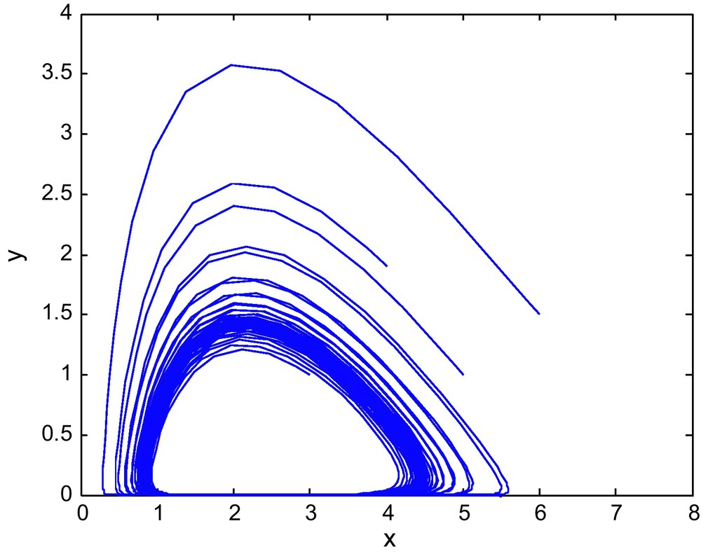
The phase diagram for (E1, E2) = (0.9, 2.69) with d = 0.9.
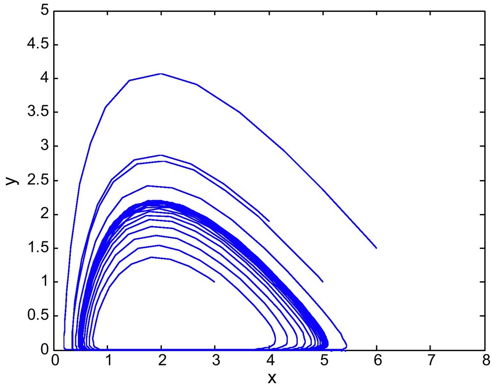
The phase diagram for (E1, E2) = (0.9, 2.69) with d = 1.0.
Figs. 7 and 8 shows the phase diagram of prey and predator with a fixed value of E2 = 2.69 and different values of E1. Fig. 9 has E1 = 0.39, and E2 = 3.60
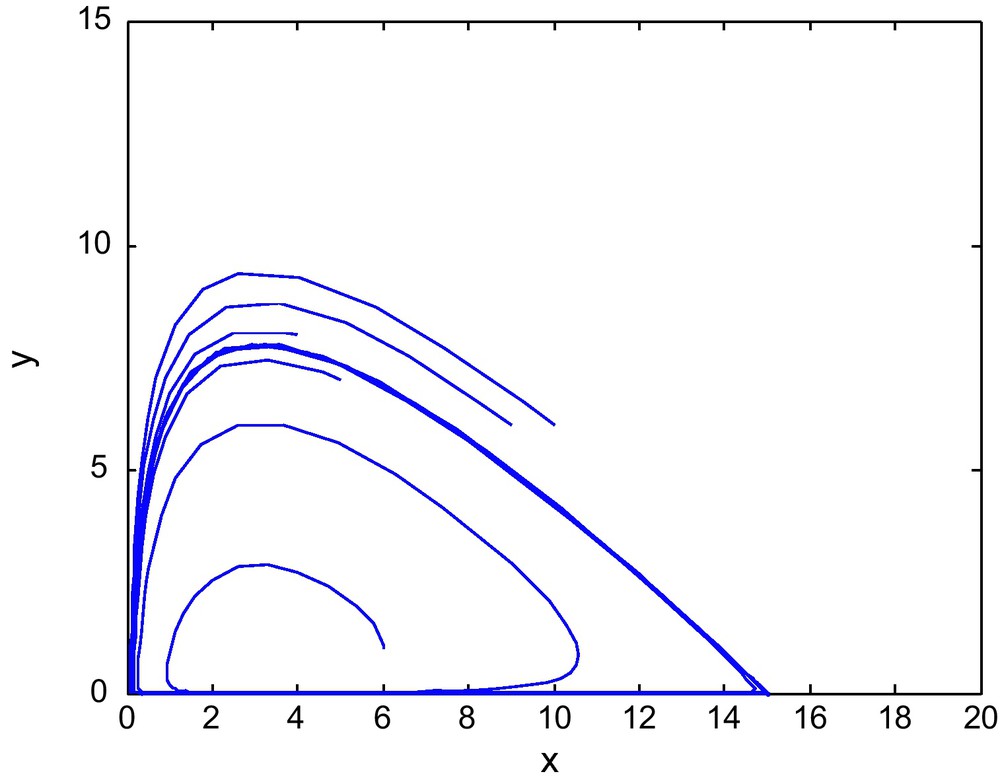
The phase diagram for (E1, E2) = (0.75, 2.69) from region-II of the Fig. 1.
The phase diagram for (E1, E2) = (2, 2.69) in region-III of Fig. 1.
The phase diagram for (E1, E2) = (0.39, 3.60) in the Region IV of Fig. 1.
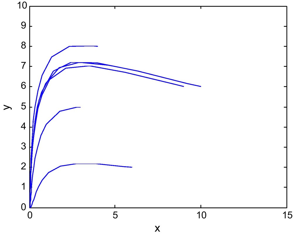
Figs. 10 and 11 shows the isoclines of prey and predator with a fixed value of E2 = 2.69 and different values of E1. It is observed that the equilibrium point for the prey population gradually decreases when the respective fishing effort used to harvest prey population is simultaneously increased. In Fig 10, d = 0.6 and in Fig. 11 d = 0 (Figs. 12 and 13).
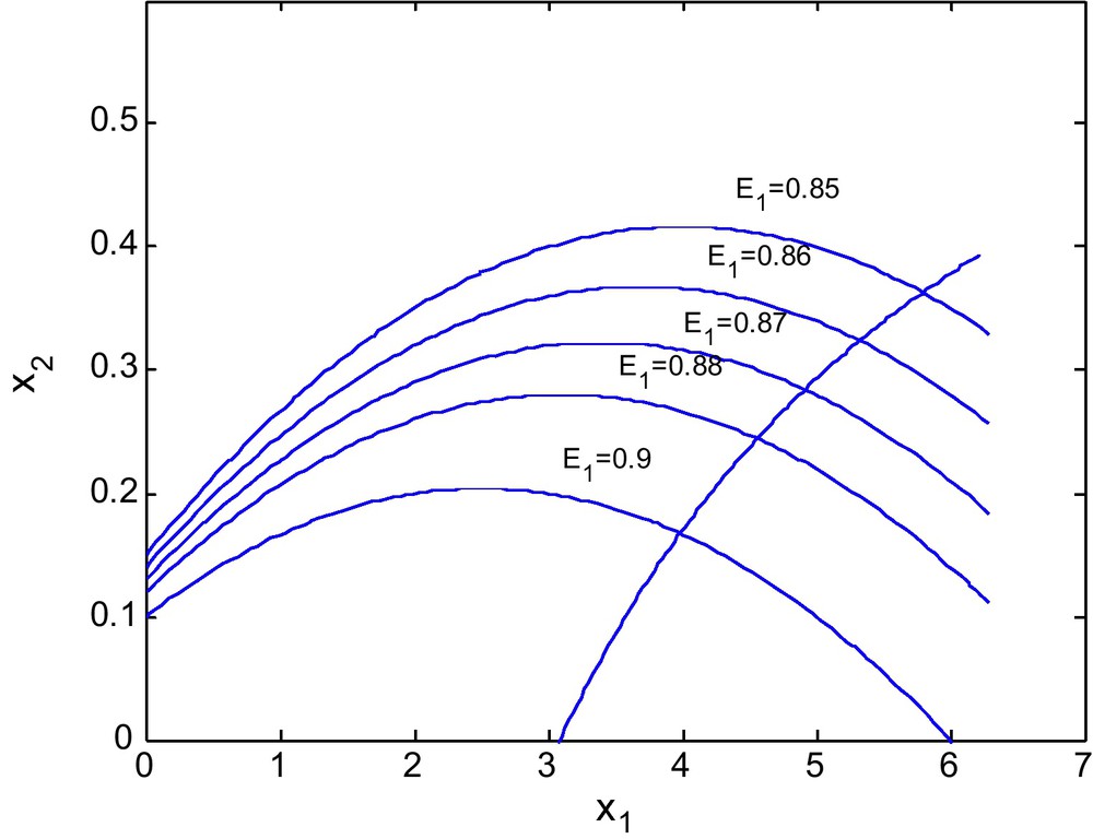
For d = 0.6.
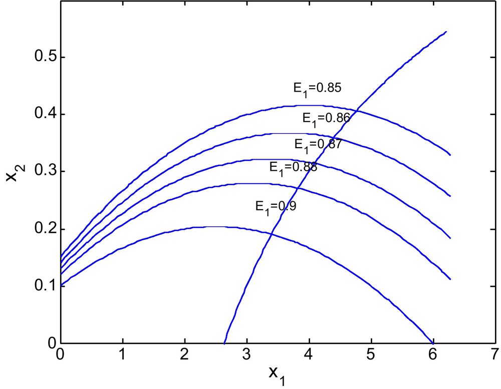
For d = 0.
For d = 0.6.
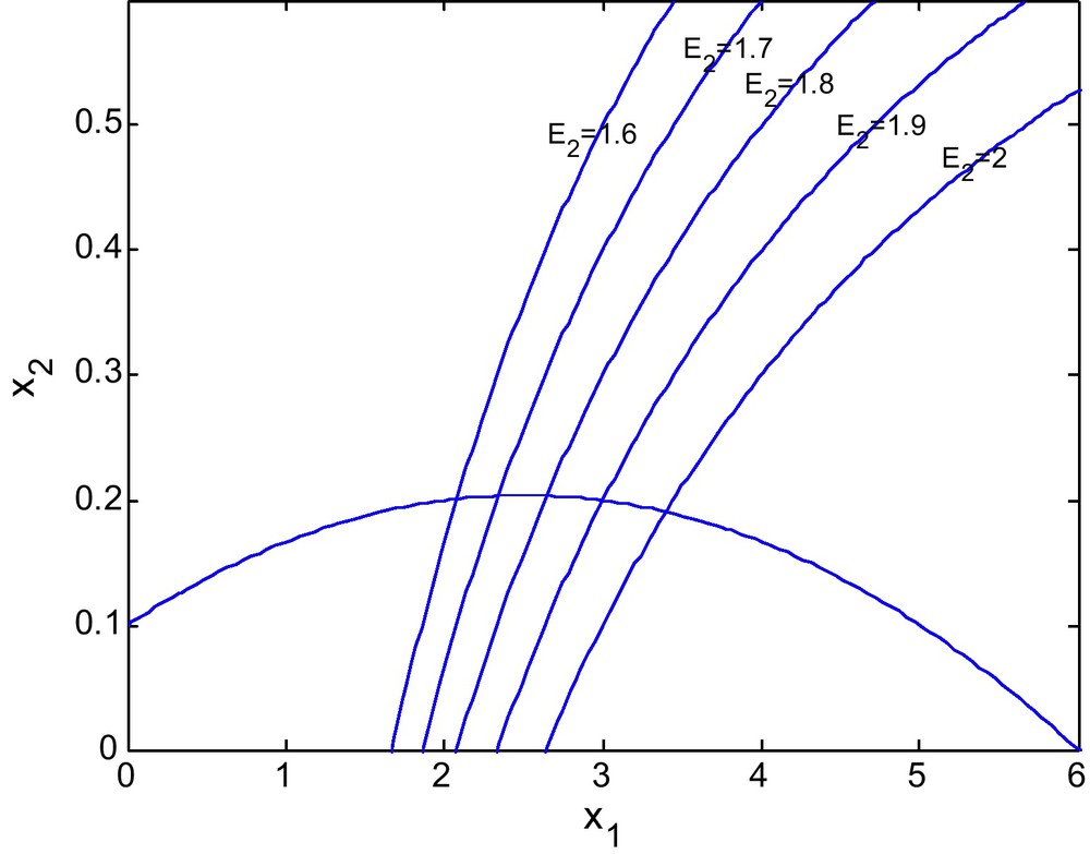
For d = 0.
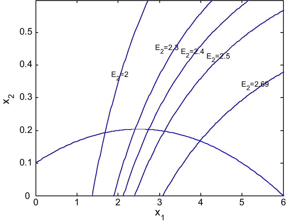
Figs. 12 and 13 show the isoclines of prey and predator population with a fixed value of E1 = 0.6 and different values of E2. It is observed that the equilibrium point for the prey population gradually increases as the effort E2 increases. It is natural as an increase in E2 decreases the predator population and hence enhancing the survival rate of the prey.
5 Conclusion
Managing predator-prey systems involves complex challenges for resource managers. Many studies have demonstrated populations consequences of predators on prey population, but how managers should use this information are not easy to decide. Predator control can be effective at enhancing survival and recruitment in populations of prey, but the potential role of predators in structuring ecological communities has been recognized for sometime. For example, overexploitation of sea otter populations resulted in increase in sea urchins that subsequently destroyed kelp beds that provided habitats for fish and other marine organisms. Because of such complexity of food webs in ecological communities it is difficult to anticipate the full ramifications of eliminating or restoring predators. For example, reducing predator numbers to increase abundance of prey can have counter-productive results such as increasing disease and parasite infection in prey.
We believe that prey-predator management requires ecosystem management and this must include careful consideration of habitats as well as the particular predator prey populations. Management actions include adjusting season length and bag limits for hunter and trappers, but must also include other activities such as management of habitats that provide secure areas for prey. Ecosystem management acknowledges the value of predators in the environment.
Thus unregulated exploitation and extinction of many natural and biological resources is a major problem of present day. This work pays attention to the exploitation or harvesting of such resources. It describes some strategies on harvesting efforts of a prey-predator model incorporating an alternative prey for the predators. It gives a study of a prey-predator model with an alternative prey, which shows some methods to control the system and how the state can be driven into equilibrium. We have considered all possible cases for the variation of parameters for the equilibrium and stability analysis of the model. It has also been discussed, how the system bifurcates from equilibrium. We have seen that the interior equilibrium in Case 3 is stable for E1 > ϕ(E2) and is unstable for E1 < ϕ(E2) and another interior equilibrium is always unstable. Some numerical examples also show how the system becomes stable at an interior equilibrium and how it bifurcates from the equilibrium and also some other features of the model.
Managing prey-predator populations for hunter harvest becomes more complex when predators are competing with humans for the same prey. Adjustments to harvest regimes may be necessary, but certainly we can have sustainable harvest of populations under predation. Elk on the northern range of Yellowstone National Park are harvested by hunters when they move into Montana during winter. The sustainability of this harvest is ensured because the Montana Department of Fish, Wildlife and Parks has density dependent harvest guidelines so that the number of tags issued for the late-Gardiner elk hunt increases with the number of elk censused on the northern range. This helps to balance the hunter harvest with wolf predation ensuring that the elk population is not driven to low levels by excessive hunter harvest.
Model that has been developed permit harvest guidelines while accommodating predators and these can be used to achieve sustainable yields. However application of this model will require data to manage a prey-predator systems.