

1 Introduction
Freshwaters, which are rapidly deteriorating all around the world, have been the focus of more and more attention [1–3]. This attention has inspired many studies analyzing the ecological, environmental and habitat factors that affect the distribution of freshwater organisms at different spatial scales. However, one kind of freshwater organism that has been relatively neglected is the crustacean [4–9]. In relation to crustaceans, we endeavored to analyze the relationship between species distribution and ecological factors, a fundamental step towards increasing our knowledge of freshwater ecosystems, of the communities associated with them, and of information important for management and conservation. Worldwide, freshwater habitats are being subjected to such marked human disturbance that the extinction rate of freshwater species is predicted to be five times that of terrestrial species and three times that of coastal marine mammals [10]. All this hastens us to foster habitat and species preservation by developing practical tools for assessing running waters and species conditions ecologically.
The biological model we used in this research project is the white-clawed crayfish Austropotamobius pallipes complex, the biggest indigenous freshwater invertebrate in Western and Central Europe [11,12]. Over the last few decades, European populations of native crayfish have been fragmented and have declined all over the continent [13]. Human disturbance has provoked habitat fragmentation, deforestation and water deterioration. Larger, more aggressive, and quicker-growing non-native crayfish [14–17] have been introduced. On top of this, human disturbance is liable to become even more severe in the future while non-indigenous species are transmitting the crayfish plague due to Aphanomyces astaci (Schikora, 1906) [18].
Obviously, A. pallipes has been in need of special protective measures and so was listed as “vulnerable” on the Red List of threatened animal species compiled by the International Union for the Conservation of Nature and Natural Resources [19] and in annexes II and V of the Habitat Directive (Council of the European Communities, 1992, 1997). In Piedmont (NW Italy), A. pallipes is protected locally by a Regional Law (L.R. number 37 dated 29/12/06), which lays down new regulations for the management of aquatic fauna, habitat, and fishing. In particular, it provides policies aimed at re-establishing consistent populations of native species.
A. pallipes, like other native crayfish, is considered a keystone species [20], an important component of many food webs in freshwater ecosystems [21–24]. Crayfish are involved in the food chain: they are prey for vertebrate predators [25] and, in turn, are omnivorous feeders with a significant impact on community structures [26–31]. They play an important role in the well-being of running water ecosystems [32] and take part in the cycling of matter and the flow of energy [33]. Although A. pallipes have long been considered valid bioindicators of water quality [34–36], they also inhabit moderately polluted waters [8,9,37]. These were the factors that have led us to investigate the relationship between the environment and the presence/absence of A. pallipes.
In our research project, we have used modeling, a tool being considered more and more important for defining management and conservation policies. Ecosystems have highly complex nonlinear relationships among their input variables, and so researchers have been applying machine-learning methods to ecology in the last decade [38–46]. One reason is that machine-learning techniques introduce fewer prior assumptions about the relationships among the variables and hence are better than traditional statistical analysis in many ways. There are many machine learning techniques. However, decision trees [47], artificial neural networks [48], fuzzy logic [49], and Bayesian belief networks [50] are the techniques that seem to model habitat suitability the best [41,51].
Our research project evaluates the reliability of various current classification techniques in modeling A. pallipes presence/absence and ranks their performances. We used two types of approaches. Firstly, we used the multivariate-statistics approach, where we applied logistic regressions (LRs). Secondly, we used the machine-learning approach, where we applied decision trees (DTs) and artificial neural networks (ANNs). These types of machine-learning techniques have been used at various rates – ANNs quite often from mid-1990s [44–46,48,52–62], DTs sporadically [41,45,46], and LRs most frequently [56].
2 Material and methods
2.1 Study area and data collection
We chose sites for sampling A. pallipes distribution on the basis of both recent information and historical records – by examining the literature, by collecting information from museums, and by contacting local town administrators, natural-park and wildlife-reserves personnel, and local people. The 175 sites we chose covered a total area of 25,399 km2 and were located along brooks and small tributaries flowing into the Po River. They mostly were characterized by running waters inhabited by native crayfish in the past. We performed samplings from late spring to early autumn 2005–2009 in all 8 provinces of Piedmont Region: Alessandria, Asti, Biella, Cuneo, Novara, Verbania, Vercelli, and Torino.
The sites had geological conditions typical for Piedmont, ranging from the siliceous to the calcareous, and therefore widely varied in their physical and chemical characteristics. Species presence was assessed both during the day performing manual surveys (2 people for 1 hour) and at night using traps (50 × 25 × 25 cm with a 3 mm mesh size, baited with pig or chicken liver, left overnight). Each site was sampled three times before considering it not inhabited by the crayfish.
2.2 The choice of input variables
The more the parameters used, the more complex the models are, the greater the calculation times, the greater the field data collection efforts, and – unfortunately – the more obfuscated the models. Accordingly, we chose only a few variables, those most important for detecting A. pallipes presence, as reported [8,9,15].
2.2.1 Environmental variables
Some stream characteristics were considered in situ: altitude; width at moderate flow; width at high flow; percentages (0–100%, not classes) of the sampled area classified according to granulometry-bedrock, boulders and pebbles, medium gravel (≥ 1 cm), little gravel (1 cm < dimension ≤ 2 mm), sand and silt (dimension < 2 mm); water velocity; and amount of shade (classes 0–5; the larger the shade, the larger the value).
2.2.2 Physical-chemical variables
In each site we measured pH, conductivity (C) and percentage of dissolved oxygen (DO) through a multiparameter probe (mod. Hydrolab Quanta). To avoid floating materials, we set a 15 cm depth for collecting two 100 mL water samples from each site. We stored the samples in sterile polythene test tubes and froze them until they were analyzed chemically. We measured the concentrations of the following inorganic ions that are commonly used to assess water quality: ammonium (NH4+), nitrates (NO3−), ortho-phosphate (PO43−), chlorides (Cl−), sulfates (SO42−), calcium (Ca2+), and magnesium (Mg2+). To do this, we used a spectrophotometer Dr Lange Lasa 100 following IRSA [63]. Then the BOD5 was evaluated, as in Lenor et al. [64]. Generally, ion concentrations are not conservative variables. However, the reason why we used them was that the samplings were always performed during normal flow regimen from late spring to early autumn. Therefore the ion concentrations that were measured were assumed to be constant.
2.2.3 Climate variables
We used the software DIVA-GIS version 5.4.0.1 (http://www.diva-gis.org) with raster data taken directly from BIOCLIM. This is a bioclimatic prediction system that approximates energy and water balances at given locations by using surrogate terms (bioclimatic parameters) derived from mean monthly climate estimates [65]. In effect, BIOCLIM uses monthly or weekly values of maximum temperatures, minimum temperatures, rainfall, radiation, and evaporation to derive bioclimatic parameters. We used the following terms: annual mean temperature (the mean of all the weekly mean temperatures; each weekly mean temperature = the mean of that week's maximum and minimum temperature), maximum temperature of the warmest period (the highest temperature of any weekly maximum temperature), minimum temperature of the coldest period (the lowest temperature of any weekly maximum temperature), annual precipitation (the sum of all the monthly precipitation estimates), precipitation of the wettest period (the precipitation of the wettest month), and precipitation of the driest period (the precipitation of the driest month).
2.3 Data-set pre-processing
Data was normalized proportionally before we use a data set to build the different models. We normalized as in Tirelli et al. [46]. In addition, we selected attributes by applying different feature selection techniques. In general, features are selected by searching the space of attribute subsets, something accomplished by combining an attribute-subset evaluator with a search method. In our case, we used filter methods, which select features on the basis of measures of feature predictability and redundancy. Supervised filters are very flexible and allow various search methods and evaluation methods to be combined. We chose five supervised filter evaluators to find the best feature set (χ2, Information Gain, Gain Ratio, Symmetrical Uncertainty, and OneR), all available in WEKA [66], along with one search method (Ranker). We used the 10-fold cross-validation for each of the five methods. We used the missing-merge option for each of the evaluators, an option that allows users to distribute counts for missing values, which are distributed across other values in proportion to their frequency.
We used three options for the Ranker search method: (a) generate ranking, a constant option of this method; (b) number to select, which allows the user to specify the number of attributes to retain; the number we used was the default value (−1), which neither excluded any attribute nor reduced the attribute set; and (c) threshold, which allows users to set the threshold beyond which attributes can be discarded. We used threshold at default value because it is the option according to which no attributes are discarded.
The algorithms used in each evaluator are those described in detail by Witten and Frank [66]. These are techniques that search among the attributes for the subsets most likely to predict the class. Through them, we obtained the following unique core of 15 inputs: (1) PO43−, (2) NH4+, (3) NO3−, (4) Ca2+, (5) BOD5, (6) DO percentage saturation, (7) pH, (8) conductivity, (9) % of bedrock, (10) water velocity, (11) amount of shade, (12) width at moderate flow, (13) altitude, (14) minimum temperature of coldest period, and (15) precipitation of wettest period. This is the unique core of variables that is essential for contrasting the performances of the different models. We acknowledge that the selection of variables is not necessarily independent of the modeling approach (e.g. a variable that can be effective with ANNs may be ineffective with DTs). Nevertheless, we used the same set of variables to contrast the performances of the different models.
2.4 Analyses
2.4.1 Logistic Regression and Principal Component Analysis Classification
We performed Logistic Regression (LR) to distinguish sites inhabited (positive sites) by A. pallipes complex from sites not inhabited by them (negative sites). We carried out multivariate analyses using Principal Component Analysis (PCA) and LR (following the procedure suggested by 56). PCA used the 15 inputs from feature selection, so that the positive correlated variables were transformed into a smaller number of variables (principal components [PCs]). This coordinate transformation reduced the redundancy within the data by creating a new series of components. These principal components were linear combinations of the original response vectors and were chosen because they contained the most data variance and because they were orthogonal. We assessed how much we could separate positive sites from negative ones. To do this, we conduced LRs, only using PCs with eigenvalue > 1. We performed these analyses by employing the stepwise-forward-selection entry of independent variables. We used species presence/absence as the dependent variable and the PCs as independent variables [9]. We estimated a reliable error of the models by estimating the performances of LRs from a leave-one-out jackknifing involving a holdout procedure repeated 10 times and using a model derived from a calibration set of 80% of the sites. In turn, this model was applied to the remaining test sites [46,56]. We calculated the average predictive performance and chose, as the final model, one of the 10 LRs included within this range.
2.4.2 DT models
We induced rules in the form of decision trees using a common technique [47], the top-down induction of decision trees. These rules related the values of the inputs to the presence/absence of white-clawed crayfish. We used the J48 algorithm with a binary split. J48 is the Java re-implementation of the C4.5 algorithm [67], one of the most well-known and widely used decision-tree induction methods. We decided to use a binary split on the basis of the papers by Dakou et al. [41] and Tirelli et al. [46], both of whom obtained positive results in a freshwater context. The outputs of the models are discrete variables (presence or absence of A. pallipes), but all the inputs are continuous.
We applied the tree-pruning optimization method both in order to reduce the effects of noise in the data and the complexity and to improve the accuracy of the predictions. Tree pruning is a common way to cope with tree complexity. Optimal tree pruning eliminates errors from data noise and therefore reduces the size of models and makes them clearer and more accurate in their classifications [68]. We used post-pruning with the intensity controlled by changing the confidence factor (a parameter affecting the error rate estimate in each node) between 0.15 and 0.25.
To assess model performances, we evaluated five parameters on the basis of matrices of confusion [69]: (1) the percentage of Correctly Classified Instances (CCI), frequently used when presence/absence of taxa is predicted; (2) model sensitivity (the ability to predict species presence accurately); (3) model specificity (the ability to predict species absence accurately); (4) Cohen's kappa coefficient [70]; and (5) the area under the receiver-operating-characteristic (ROC) curve.
The CCI are affected by the frequency of occurrence of the organism being modeled [68,71]. Thus Cohen's k coefficient, being negligibly affected by prevalence, is a more reliable performance measure of presence/absence models [72–74]. Cohen's k gives a rather conservative estimate of prediction accuracy because it underestimates agreements due to chance [75]. However, k values come from the information content of the dataset, which has limited extractable information. For this reason, there may be differences in k threshold values according to the discipline, according to Gabriels et al. [76]. These are the researchers who have assessed the following k values in a freshwater ecological context: 0.00–0.20: poor; 0.20–0.40: fair; 0.40–0.60: moderate; 0.60–0.80: substantial; and 0.80–1.00: excellent. In the area under the ROC curve, Hosmer and Lemeshow [77] suggest that 0.7 indicates satisfactory discrimination, 0.8 good discrimination, and 0.9 very good discrimination.
Model training and validation were based on stratified 10-fold cross-validation [78]. To estimate a reliable error of the models, we repeated 10-fold cross-validation experiments 10 times and we calculated the average predictive performance. The Mann-Whitney U tests were carried out to contrast the performances of the unpruned and pruned models as well as of DTs and LRs. Comparisons were made on the basis of the parameters mentioned above.
2.4.3 ANN models
We used sites that tested both positive and negative for crayfish. We employed all the measured parameters and thereby built a model using a feed-forward multilayer perceptron trained by the back-propagation error algorithm [75], a very common training method [43,45,46,80]. We built a three-layered feed-forward neural network with bias and developed it with an architecture that is described as follows. There were 15 input nodes, the 15 features resulting from the feature selection. There was only one output node – crayfish presence/absence. There was one hidden layer between the input and the output layers. In this hidden layer, the number of neurons was optimized by trial and error. We chose this single layer because a single layer generally shortens computation times and often yields the same results as ANNs with more than one hidden layer [81,82]. We chose the number of hidden neurons to minimize the trade-off between network bias and variance [82], and determined the optimal number empirically by contrasting the performances of different ANNs. We tested a range of architectures with variations in momentum (range 0.1–0.5), learning rates (range 0.1–0.5), epochs, and number of neurons in the hidden layer. We did this until we obtained the best predicting models. Then we examined models with similar performances and chose the simplest of them – those with the fewest hidden nodes. Simple models are more useful for two reasons. First, the simpler of two similar networks is the one more likely to predict new cases better [82]. Second, the best of all network geometries is that of the smallest network that captures the relationships in the training data adequately [74]. Cross-validation is particularly useful when the number of cases is limited. We therefore used cross-validation to avoid over-training the networks and used the error back-propagation algorithm [79] to train cross-validated neural networks. We assessed the performance of predictive models using the same five parameters on the basis of the matrixes of confusion [69] already mentioned for DTs.
Model training and validation were based on stratified 10-fold cross-validation [78]. In order to estimate a reliable error of the models, 10-fold cross-validation experiments were repeated 10 times. Finally, we calculated the average predictive performances and chose one of the 10 networks included within this range as the final network for our model. We performed the Mann-Whitney test to contrast the performances of the ANN models with DTs and models with LRs. We did not use a dedicated test set because the amount of data available was limited [46].
3 Results
3.1 Crayfish distribution
Detected streams showed extensive habitat wealth. Some of the sampling sites were greatly affected by human activities (25.14%) while others were not. The areas of high anthropic impact were characterized by discharges and by the modification of landscape features. Most anthropic impact came from farms, factories, and sewers. Most of the landscape modifications were due to plantation, canalization, dredging, reservoirs, and engineering work. Native crayfish populations were not found in 77 (44.00%) watercourses, but were found in 98 (56.00%). Fig. 1 shows the distribution of both the positive and the negative sampled sites.
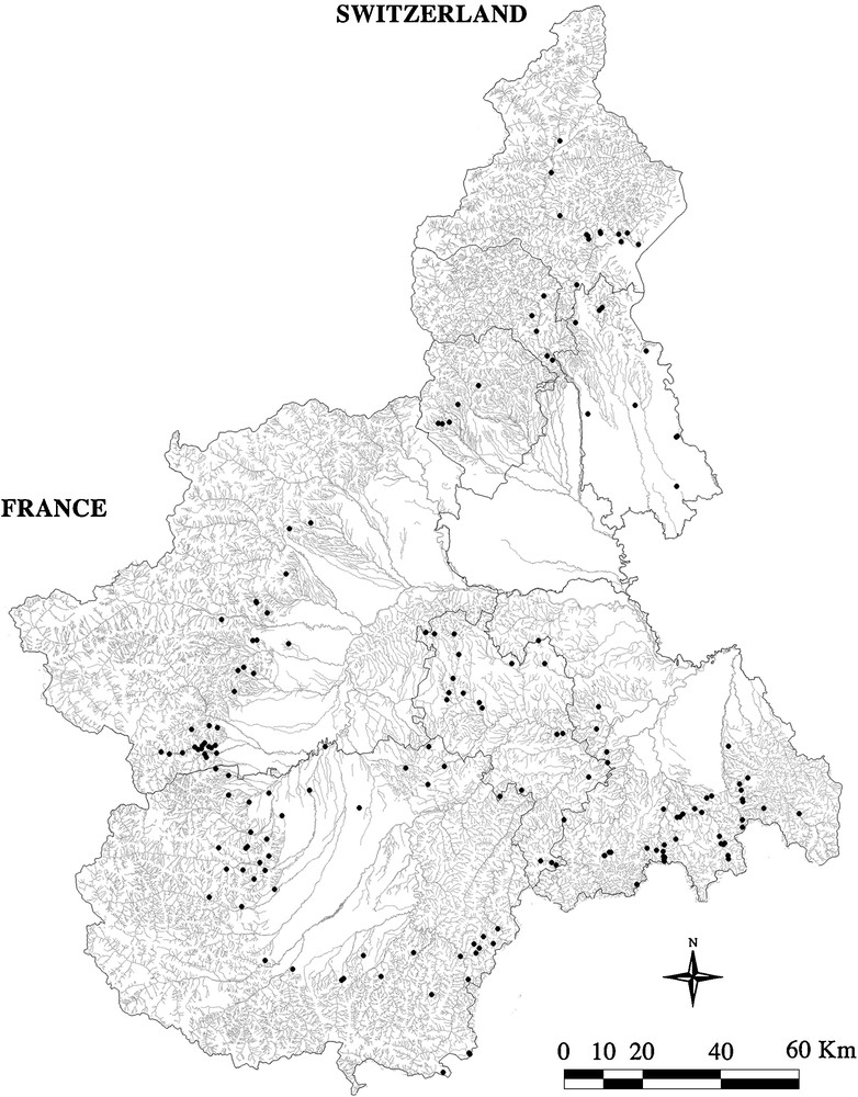
Map of the Piedmont region showing the distribution of the 175 sampling sites.
3.2 PCA and LR classification
PCA showed that the total variance of all 6 components with eigenvalue > 1 ranged up to 68.36% (Table 1). The mean performances and standard deviations of LRs were calculated on models built using the 6 PCs with eigenvalue > 1. Mean LR models correctly classified 67.96% of the sites – 74.81% of the sites with crayfish presence and 59.02% of the sites with absence. The best performing LR model showed the best classification results when it had three PCs (PC2, PC3, and PC4) and when these were retained in the equation at the step 3 (Table 2). Overall, this model correctly classified 74.60% of the sites – 86.00% for presence and 57.10% for absence (Table 3).
Weight of each one of the 15 selected variables in building the principal components (PCs).
| PCs | ||||||
| 1 | 2 | 3 | 4 | 5 | 6 | |
| Eigenvalue | 3.10 | 2.08 | 1.70 | 1.27 | 1.11 | 1.01 |
| % of variance | 20.66 | 13.86 | 11.34 | 8.45 | 7.39 | 6.67 |
| Conductivity | 0.678 | −0.133 | 0.249 | 0.388 | 0.113 | 0.114 |
| Ca2+ | 0.665 | −0.005 | 0.251 | −0.357 | 0.061 | −0.205 |
| Dissolved oxygen [% of saturation] | −0.642 | −0.040 | 0.119 | −0.287 | −0.058 | −0.154 |
| Altitude | −0.578 | 0.413 | 0.103 | 0.151 | −0.064 | 0.350 |
| Minimum temperature coldest period | 0.564 | −0.271 | 0.542 | −0.063 | −0.101 | 0.175 |
| Water velocity | −0.541 | 0.029 | 0.225 | −0.183 | 0.261 | 0.326 |
| Precipitation wettest period | 0.074 | −0.663 | −0.133 | 0.381 | −0.171 | −0.143 |
| NH4+ | 0.407 | 0.648 | 0.113 | 0.315 | 0.074 | −0.101 |
| PO43− | 0.221 | 0.584 | 0.247 | 0.130 | 0.427 | 0.207 |
| BOD5 | 0.011 | 0.521 | −0.234 | 0.406 | −0.271 | −0.360 |
| pH | 0.128 | 0.150 | 0.686 | −0.214 | −0.457 | −0.026 |
| Width at moderate flow | −0.363 | −0.325 | 0.565 | 0.263 | 0.161 | −0.231 |
| % of bedrock | −0.429 | −0.308 | 0.273 | 0.552 | −0.030 | 0.227 |
| NO3− | 0.335 | −0.337 | −0.278 | −0.034 | 0.543 | 0.055 |
| Shade | 0.419 | −0.072 | −0.344 | −0.010 | −0.430 | 0.593 |
Results of the logistic regressions (LRs) for principal components (PCs).
| B | S.E. | Wald | df | P | Exp (B) | ||
| Step 1 | PC2 | −0.549 | 0.182 | 9.090 | 1 | < 0.01 | 0.578 |
| Constant | 0.451 | 0.179 | 6.380 | 1 | < 0.05 | 1.570 | |
| Step 2 | PC2 | −0.611 | 0.194 | 9.881 | 1 | < 0.01 | 0.543 |
| PC3 | −0.517 | 0.191 | 7.290 | 1 | < 0.01 | 0.596 | |
| Constant | 0.424 | 0.183 | 5.363 | 1 | < 0.05 | 1.529 | |
| Step 3 | PC2 | −0.613 | 0.194 | 10.004 | 1 | < 0.01 | 0.542 |
| PC3 | −0.526 | 0.193 | 7.429 | 1 | < 0.05 | 0.591 | |
| PC4 | 0.378 | 0.187 | 4.061 | 1 | < 0.05 | 1.459 | |
| Constant | 0.430 | 0.187 | 5.285 | 1 | < 0.05 | 1.537 |
Classification table of logistic regression (LR) for the 6 principal components (PCs).
| Overall (%) | Presence (%) | Absence (%) | |
| Step 1 | 59.9 | 83.7 | 23.2 |
| Step 2 | 66.2 | 84.9 | 37.5 |
| Step 3 | 74.6 | 86.0 | 57.1 |
3.3 DT models
The average and standard deviations of the five performance parameters were calculated both for unpruned and post-pruned DTs (Table 4). The unpruned trees had very many leaves, which made them more complex and hindered ecological interpretations (Table 4). Pruning usually makes models less complex and makes their performances more efficient. Thus, models with different intensities of post-pruning were induced by varying the confidence factor between 0.15 and 0.25. The optimal confidence factor was 0.15. The percentages of CCI and Cohen's k statistic were quite low in all the cases. Cohen's k statistic made the models reliability poor. The values obtained by Cohen's k revealed that most of the predictions were based on chance. Sensitivity always reached quite high values (> 73.0%), while specificity was only 55.5%. The area under the ROC curve (0.7) indicated satisfactory discrimination. The best performing DT from among these 10 inputs had CCI = 72.45%, Cohen's k = 0.43, sen = 80.33%, spe = 62.50% and area under the ROC curve = 0.71.
Predictive results of decision tree models based on the J48 algorithm without pruning and with post-pruning optimization.
| DTs with binary split | CCI | k | sen | spe | ROC | # l | c.f. | |
| Unpruned | Mean | 65.3 | 0.30 | 73.0 | 55.5 | 0.7 | 18.6 | 0.18 |
| s.d. | 2.8 | 0.06 | 3.8 | 4.2 | 0.03 | 1.5 | ||
| Pruned | Mean | 65.9 | 0.30 | 74.4 | 55.5 | 0.7 | 15.7 | 0.15 |
| s.d. | 3.4 | 0.07 | 4.0 | 4.6 | 0.03 | 1.3 | ||
| Mann-Whitney | P | n.s. | n.s. | n.s. | n.s. | n.s. | < 0.001 |
We performed the Mann-Whitney U test to contrast the five parameters (CCI, model sensitivity, model specificity, Cohen's kappa coefficient, and the area under the ROC curve) used to assess performances and the mean number of leaves between pruned and unpruned models. No significant differences in the predictive performances were detected, while a significant difference was found in the number of leaves. For this reason, we will only consider pruned trees for further comparisons.
Moreover, the Mann-Whitney U tests were carried out to compare CCI, model sensitivity, and model specificity in LR and in pruned-DT models. There were no significant differences in their predictive performances (P > 0.05).
3.4 ANN models
The optimization of the number of hidden neurons by trial and error resulted in the following network architecture: 15 input neurons, 8 hidden neurons and 1 output neuron. The learning rate was set to 0.3, the momentum set to 0.2, and the maximum number of epochs to 400. We calculated the average and the standard deviation of the five performance parameters of the 10 repeated 10-fold cross-validated ANNs (CCI = 72.99%, k = 0.45, sen = 75.16%, spe = 70.18%, ROC = 0.80). We chose the final network from among these 10 ANNs. This network had quite a high percentage of CCI (78.95%), of sensitivity (79.56%), of specificity (78.04%), a moderate k coefficient (0.57) [78] and an area under the ROC curve of 0.81. This area of 0.81 indicates that the model discriminates well [77].
We performed the Mann-Whitney U test to compare the performances of DT and ANN models. ANNs performed better than DTs (P < 0.05), except for sensitivity (P > 0.05). We carried out the Mann-Whitney U test to compare the performances of the LR and the ANN models. The tests showed that ANNs performed better than the LRs (P < 0.001), except for sensitivity (P > 0.05). The final ANN model was influenced by all the 15 inputs used to model the presence/absence of the species in Piedmont. This illustrates that if we choose the features accurately, those features that we retain are the only effective inputs.
4 Discussion
The most obvious finding of our research project is that A. pallipes is distributed across Piedmont in a heterogeneous and fragmented way (as it is in the Lazio Region in central Italy [16]). Over the last few decades, populations of A. pallipes declined considerably in Piedmont [83], as in all of Europe [12,13,18,84,85]. We no longer observed crayfish in 77 previously inhabited watercourses probably because there has been habitat fragmentation, engineering work, stream canalization, deforestation, and increased water pollution.
We have endeavored to determine the predictive model that performs the best because such a model can be used to manage and protect endangered species better. Not all the modeling procedures we tested performed well. LR models performed as they did in the tests of Manel et al. [56]. ANNs outperformed both LR models and DT models. LRs performed worse in relation to specificity than in relation to sensitivity probably because there were more sites with crayfish presence than absence. DTs performed the worst of all. Cohen's k statistic showed that DT models yielded unreliable predictions, in that most of the classifications were based on chance, as they did in previous studies where they did not perform well in predicting macroinvertebrates [41]. In Dakou et al. [41], Cohen's k values were even lower than those in the present study. The unpruned DTs were too complex with their many leaves to yield any ecological interpretation. The J48 algorithm produced very detailed trees that prevented the models from generalizing any more. Therefore we used post-pruning to reduce tree complexity and variance. Post-pruning did not make the models perform better, as in Tirelli et al. [46] and Tirelli and Pessani [45]. However, they did yield simpler trees that could be interpreted ecologically [41,45,46].
Learning in ANNs is sensitive to the input data used. When researchers choose the appropriate features through pre-processing, their models perform considerably better in ecological contexts [46]. When there is no variable selection in ANNs, irrelevant information passes through the nodes, influences the connection weights slightly, and affects the overall performance of ANNs. On the other hand, variable selection decreases ANN size, reduces computational costs, increases speed, and uses less data to estimate connection weights efficiently. Feature selection eliminates all but the most relevant attributes, reduces the number of input variables, and helps models predict better [46,74,86]. In general, predictions are more accurate when the number of presences and absences is around 50% [87]. This is obviously a problem, especially when modeling rare species. It is especially important to predict presences correctly and to have accurate models when we need to predict the presence of scarce species. Such accuracy helps conserve and manage the species by identifying the potential protected areas. With this in mind, the ANN approach is valuable for modeling A. pallipes presence.
4.1 Physical-chemical variables
One finding our research project that seconds earlier research is that the organic matter dissolved in the water is a factor crucial for explaining the white-clawed crayfish distribution (all models use BOD5) [8,9,88,89]. Broquet et al. [15] and Trouilhé et al. [8] underlined that organic matter is one of the most important features of brooks with native crayfish. Vegetal residues and organic detritus are of great importance for the crayfish diet. In fact, they are the most important sources of energy and food available in freshwater ecosystems [31,90]. In our project, the BOD5 index was used to measure the organic matter that can be biologically attached by bacteria [9,15]. In addition, we built models using several other physical-chemical variables that have already been reported to be important for A. pallipes distribution [7–9]: the pH, the concentration of Ca2+, the concentration of NO3−, the percentage of dissolved oxygen in water, and the level of conductivity. Ca2+ is especially important for determining the occurrence of crayfish because it is essential for exoskeleton calcification. NH4+ and PO43− and the pollution they cause do not affect A. pallipes presence. In fact, these ions are often found in streams inhabited by A. pallipes [8,9,15,37,89,91,92]. Mean value and standard deviation of the physical-chemical variables characterizing sites inhabited by this species are reported in Favaro et al. [9].
4.2 Environmental and climate variables
Another finding that our research project supports is that A. pallipes need to avoid potential predators, extreme temperature ranges, and extreme changes in the flow of water. Thus the environmental features that can help explain their distribution are the ones that play a role in their avoiding these circumstances: (1) shade due to canopy cover and bedrock used as shelter from potential predators; (2) temperature variations (a minimum temperature during cold seasons) and temperature variations due to altitude (a good integrator of the thermal conditions); (3) scarcity or flooding of flowing water (precipitation during the wettest period and water velocity). The availability of shelters and borrows in a stream – critical for the survival of adults – is the most important resource bottleneck in crayfish populations [7,93]. This association of canopy cover with A. pallipes presence has been supported by Smith et al. [4], Naura and Robinson [5], and Broquet et al. [15], but not by Barbaresi et al. [7].
Mean value and standard deviation of the environmental and climate variables characterizing the elective habitat of A. pallipes in Piedmont are reported in Table 5.
Maximum (max) and minimum (min) values, mean (m) and standard deviation (s.d.) of the environmental and climate variables characterizing the habitat of A. pallipes in Piedmont.
| Variable | Max | Min | m | s.d. |
| Altitude [m] | 700.00 | 160.00 | 471.10 | 129.51 |
| Width at moderate flow [m] | 10.00 | 0.55 | 3.42 | 2.28 |
| Water velocity [m/s] | 1.00 | 0.02 | 0.22 | 0.16 |
| % of bedrock | 75.00 | 25.00 | 35.71 | 14.76 |
| % of shade | 90.00 | 20.00 | 63.21 | 17.87 |
| Min. temperature of the coldest period [° C] | 0.90 | −3.70 | −1.16 | 1.31 |
| Precipitation of the wettest period [mm] | 151.00 | 85.00 | 114.05 | 19.39 |
In conclusion, A. pallipes are being subjected to an unprecedented crisis [11,85]. Therefore it is imperative that researchers choose the best way to take on this crisis by understanding the relationships between endangered species and their habitats more deeply. With this in mind, they can better plan conservation and management strategies. Our advice is this: researchers must first use various techniques and then contrast their performances. Our own results illustrate the advantages of contrasting various approaches. In fact our method enabled us to predict white-clawed crayfish presence in Piedmont with reasonable accuracy. It helped us choose the best model for managing A. pallipes. Had we used fewer approaches, we would have come up with a poorer model. Our research project has underlined the synergic effects of several biotic and abiotic factors on the occurrence of A. pallipes in an effort to provide information for the maintenance of natural populations and the selection of sites and streams where reintroduction strategies may be planned. We conclude with the suggestion that researchers use and contrast various techniques, as we did, in their research in other areas.
Disclosure of interest
The authors declare that they have no conflicts of interest concerning this article.
Acknowledgements
This work was funded by the Cassa di Risparmio di Torino (CRT) Foundation through the Alfieri project. We are indebted to two anonymous referees, for their helpful suggestions for improving this paper. Special thanks are due to Giulia Bemporad for her assiduous participation in samplings.