

1 Introduction
Three species of smooth-shelled mussels, Mytilus edulis L. 1758 [1], M. galloprovincialis Lmk. 1819 [2] and M. trossulus Gould 1850 [3] have been re-defined on the basis of allozyme-genotype and concurrent morphological variation worldwide [4–6]. Although hybridization occurs in virtually every known case where two of the species occur sympatrically, evidence of restriction to gene flow despite broadcast spawning and pelagic larval transport confirms the biological status of the three species [6]. M. edulis and M. galloprovincialis are present in the temperate and cold regions of both Hemispheres, while M. trossulus is confined to the boreal and sub-boreal regions [5]. Southern-Hemisphere M. galloprovincialis are allozymically and morphologically distinct from their Northern-Hemisphere counterparts, less so M. edulis [5]. All smooth-shelled mussels from Chile examined by J.H. McDonald et al. [5] were closely related to those from Argentina, the Falkland Islands and the Kerguelen Islands, and all were clustered with Northern-Hemisphere M. edulis by both their allozymic composition and their shell morphology. This result has since been challenged, with authors claiming that Chilean mussels should be considered a local subspecies of M. galloprovincialis [7]. Independently, a number of authors, e.g. [8–14], have persisted in employing the species name ‘M. chilensis’ for smooth-shelled mussels sampled in Chile, ignoring previous work [5,6] and instead following Hupé [15]. Hupé [15] mentioned the presence of M. chilensis “en la costa, en Valparaiso, etc.” and recognized that M. chilensis “tiene enteramente el aspecto del Mytilus edulis de las mares de Europa”, except that “su forma es mas aplastada”. Given the morphological variation encountered within Northern-Hemisphere M. edulis [5], it remains to be proven that the reportedly flatter shell of Hupé’s M. chilensis constitutes a character strong enough to distinguish it from M. edulis and assign it specific rank.
Evidence of invasion by alien Northern-Hemisphere M. galloprovincialis has been reported from localities in both the Northern and Southern-Hemispheres, including the northwestern and the northeastern shores of the Pacific Ocean, southern Africa, southeastern Australia, New Zealand, and Chile ([5,16–19] and references therein). Since Northern-Hemisphere M. galloprovincialis occurs in southern central Chile [16], presumably as the result of intentional introduction for aquaculture purposes [20], there is uncertainty as to the actual genetic composition of smooth-shelled mussels samples collected along the Chilean shores for a number of physiological, ecotoxicological, and morphological and even molecular genetic studies [8–14] undertaken since [5]. Because physiological response may vary considerably across Mytilus species [5], it is mandatory to ascertain the taxonomic status of the Chilean Mytilus material used prior to physiological analysis. Also, considerable morphological differences have been reported among samples of Chilean Mytilus spp. [11,14], to an extent that suggests that different species may have been present, even though the authors assumed an effect solely of environmental factors.
Here, we review the genetic and morphometric data published within the last two decades on smooth-shelled mussels from Chile, to assess the taxonomic status of populations and eventually detect more locations along the coasts of central and southern Chile where alien M. galloprovincialis may have settled. We advocate the systematic use of a genetic assay to identify smooth-shelled Mytilus material from Chile prior to their ecological, physiological or molecular study, or to any related biomonitoring survey.
2 Materials and methods
The list of smooth-shelled Mytilus samples considered in this review is presented in Table 1 and the sample locations have been reported on a map (Fig. 1). This list tentatively includes all samples from the Chilean coasts that have been genotyped at nuclear and mitochondrial markers and reported in the literature. Table 1 also includes a sample from Maullin (southern central Chile) whose genotyping at nuclear-DNA markers mac-1 and Glu-5′ is presented here for the first time. Table 1 also presents reference samples of Northern- and Southern-Hemisphere M. edulis and M. galloprovincialis genotyped at the same marker loci.
Smooth-shelled Mytilus spp. samples examined in the present review, including samples from the Chilean coastline and reference samples from Northern- and Southern-Hemisphere Mytilus edulis and M. galloprovincialis.
| Sample | N | Marker loci | Reference | |||
| Location | Coordinates | Abbreviation | Date | |||
| Chilean Mytilus spp. | ||||||
| Valdivia | 39°51′S 73°27′W | PVA | Feb. 1997–May 1998 | 55–61 | Allozymes | [7] |
| Puerto Montt | 41°33′S 72°48′W | PPM | Feb. 1997–May 1998 | 68–71 | Allozymes | [7] |
| Ancud | 41°51′S 73°50′W | PAN | Feb. 1997–May 1998 | 31–41 | Allozymes | [7] |
| Quellón | 43°08′S 73°39′W | PQE | Feb. 1997–May 1998 | 37–72 | Allozymes | [7] |
| Arauco | 37°14′S 73°19′W | Arauco | – | 109–112 | Allozymes | [10] |
| Queule | ∼39°S ∼73°W | Queule | – | 80–108 | Allozymes | [10] |
| Valdivia | ∼40°S ∼73°W | Valdivia | – | 102–116 | Allozymes | [10] |
| Calbuco | ∼41°S ∼73°W | Calbuco | – | 110 | Allozymes | [10] |
| Ancud | ∼42°S ∼74°W | Ancud | – | 99–110 | Allozymes | [10] |
| Yaldad | ∼43°S ∼73°W | Yaldad | – | 111–128 | Allozymes | [10] |
| Pto. Marin Balmaceda | ∼43°S ∼73°W | Marin | – | 99 | Allozymes | [10] |
| Punta Arenas | 53°08′S 70°55′W | Arenas | – | 100–107 | Allozymes | [10] |
| Dichato | 36°33′S 72°57′W | CHL | Oct. 1998 | 9–76 | mac-1, Glu-5′, COI | [16,21] |
| Maullin | 41°37′S 73°36′W | MAU | Jan. 1999 | 7–52 | mac-1, Glu-5′, COI | [21], present work |
| Concepcion | 36°44′S 73°08′W | CO | 1994–2009 | 19 | Me15/16, 16S | [18] |
| Colchogue | 37°03′S 73°10′W | CL | 1994–2009 | 20 | Me15/16, 16S | [18] |
| Southern-Hemisphere M. edulis | ||||||
| Yaldad Bay, Chile | ∼43°S ∼73°W | 40 | 1986 | 25 | Allozymes | [5] |
| Chiloe, Chile | 42–43°S 73–74°W | 41 | Jan. 1988 | 23 | Allozymes | [5] |
| Punta Arenas, Chile | ∼53°S ∼71°W | 42 | Jan. 1988 | 25 | Allozymes | [5] |
| Mar del Plata, Argentina | ∼38°S ∼57°W | 44 | 1985–1988 | 25 | Allozymes | [5] |
| Falkland Islandsa | 51–52°S 58–61°W | 43 | 1985–1988 | 25 | Allozymes | [5] |
| Kerguelen Islands | ∼49°S ∼69°E | 45 | July 1988 | 22 | Allozymes | [5] |
| Kerguelen Islands | 49°28′S 69°56′E | KER | June 1997 | 79–83 | mac-1, Glu-5′, COI | [21,22] |
| Southern-Hemisphere M. galloprovincialis | ||||||
| Huon River Estuary, Tasmania | ∼43°S ∼147°E | 47 | 1985–1988 | 23 | Allozymes | [5] |
| Nedlands, Western Australia | 32°03′S 115°44′E | AUS | July 1998 | 7–46 | mac-1, Glu-5′, COI | [16,21] |
| Adventure Bay, Tasmania | 43°21′S 147°22′E | ADB | Mar. 1997 | 26–28 | mac-1, Glu-5′ | [22] |
| Alonnah, Tasmania | 43°18′S 147°14′E | ALO | Mar. 1997 | 25–59 | mac-1, Glu-5′ | [22] |
| Cloudy Bay Lagoon, Tasmania | 43°25′S 147°12′E | CBL | Feb. 1997 | 5–32 | mac-1, Glu-5′, COI | [21,22] |
| Hobart, Tasmania | 42°53′S 147°20′E | HOB | Feb. 1997 | 8–31 | mac-1, Glu-5′, COI | [21,22] |
| Partridge Narrows, Tasmania | 43°24′S 147°06′E | PAR | Mar. 1997 | 25–30 | mac-1, Glu-5′ | [22] |
| Simpson's Bay, Tasmania | 43°17′S 147°20′E | SIM | Mar. 1997 | 3–40 | mac-1, Glu-5′, COI | [21,22] |
| Dunedin, New Zealand | 45°55′S 170°28′E | DUN (=NZL) | June 1999 | 6–79 | mac-1, Glu-5′, COI | [16,21] |
| Northern-Hemisphere M. edulis | ||||||
| Aarhus, Denmark | 56°10′N 10°14′E | Аархус | 1985–1988 | 11 | Allozymes | [23,24] |
| Netherlands | – | EH | – | 59–75 | Allozymes | [7] |
| Gilleleje, Kattegat | 56°07′N 12°18′E | GIL | Sep. 1996 | 16–26 | mac-1, Glu-5′ | [16] |
| Flødevigen, Skagerrak | 58°25′N 08°45′E | FLØ | Jan. 1997 | 20–47 | mac-1, Glu-5′, COIb | [16,21] |
| Grand Fort Philippe, N France | 51°00′N 02°05′E | GFP | June 1997 | 42 | mac-1, Glu-5′ | [16] |
| Northern-Hemisphere M. galloprovincialis | ||||||
| Vigo, Spain | ∼42°N ∼09°W | GV | – | 35–73 | Allozymes | [7] |
| Palavas, Western Mediterranean | 43°31′N 03°56′E | Palavas | 1988–1990 | 75–100 | Allozymes | [26] |
| Setubal, Portugal | 38°29′N, 08°56′E | STB | Sep. 1997 | 19–26 | mac-1, Glu-5′ | [22] |
| Sète, Western Mediterranean | 43°24′N 03°41′E | SET | May 1996 | 56–68 | mac-1, Glu-5′ | [16] |
| Chioggia, Adriatic Sea | 45°13′N 12°18′E | CHI | June 1997 | 18–47 | mac-1, Glu-5′ | [22] |
| Bloubergstrand, South Africa | 33°48′S 18°27′E | SAF | Nov. 1998 | 62–65 | mac-1, Glu-5′ | [16] |
| Southern Korean Peninsula | ∼35°N ∼126°E | KOR | < 1999 | 19–30 | mac-1, Glu-5′ | [16] |
| Bodega Bay, California | 38°19′N 123°04′W | BOD | Nov. 1996 | 23–34 | mac-1, Glu-5′ | [16] |
| Sète, Western Mediterranean | ∼43°N ∼03°E | G-Fr | < 1998 | 17 | 16 S | [27] |
a Sample consisting of a mixture of individuals from Stanley Harbour (51°42′S 57°49′W) and individuals from the West Falkland Island.
b COI sequences originally are from sample ‘Tjärnö, Sweden’ [25].
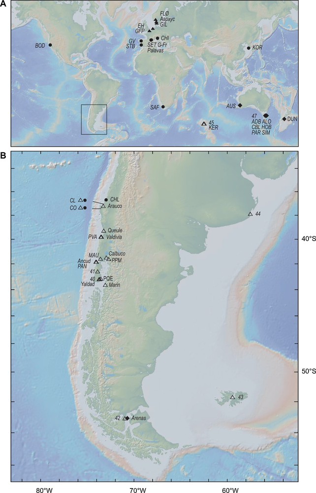
Sampling sites for smooth-shelled Mytilus spp. A. Sampling locations for Mytilus edulis and M. galloprovincialis in the Northern and the Southern-Hemispheres. B. Map of the southern tip of South America, including all sampling sites for smooth-shelled Mytilus spp. in Chile ([5,7,10,16,18,20–24]; present study). Full triangles (): Northern-Hemisphere M. edulis; full circles (): Northern-Hemisphere M. galloprovincialis; open triangles (): Southern-Hemisphere M. edulis; diamonds (): Southern-Hemisphere M. galloprovincialis. Background topographic map from GeoMapApp [28] (http://www.geomapapp.org).
C. Carcamo et al. [7] have analyzed 4 samples from the Chilean coasts, together with reference samples of Northern-Hemisphere M. edulis and M. galloprovincialis, at 23 polymorphic allozyme loci. Eight of these marker loci were common with the previously published worldwide dataset of McDonald et al. [5]. Homologies between electromorphs from different studies [5,7,23,24,26] were inferred as detailed in the legend to Appendix A.
J.E. Toro et al. [10] have analyzed 8 samples from the Chilean coast using 7 allozyme loci. Four samples (‘Ancud’, ‘Yaldad’ ‘Valdivia’ and ‘Pta. Arenas’) were from the same locations as previous allozyme surveys [5,7], potentially allowing cross-comparisons at two loci scored in common (Gpi, Pgm). Three other loci scored by [10] (GSR, ICD, ME) had not been scored by [5], and we were unable to establish correspondence between either of the remaining loci, LAP or PEP, scored by [10] and any of the Aap, Ap or Lap loci of [5] or [7]. Correspondence between electromorphs was easily established at locus Gpi, where electromorphs A and (B + C) of [10] were found to be homologous to, respectively, compound electromorphs ≤ 96 and ≥ 98 of [5] (Appendix B). Locus-Pgm electromorphs A, B and (C + D) of [10] were found to be homologous to, respectively, electromorphs < 93, 100 and ≥ 106 [5] (Appendix B). Locus Gpi shows substantial electromorph-frequency differences between Southern-Hemisphere M. edulis and M. galloprovincialis ([5]; Appendix A) and therefore Gpi is potentially helpful to assess the occurrence of alien M. galloprovincialis in Chile. We noted that allelic frequencies at locus Pgm in sample ‘Pta. Arenas’ of [10] were not consistent with those reported earlier [5].
The sample from Maullin (Tables 1, 2) was analyzed for polymorphism at nuclear-DNA loci mac-1 and Glu-5′ and compared to other samples previously analyzed using these two markers [16,22,29,32] (Appendix C). The protocols for DNA extraction, PCR amplification and electrophoresis and staining of PCR products have been detailed previously [22].
Smooth-shelled Mytilus spp. Summary of genetic characteristics at nuclear-DNA loci mac-1and Glu-5′ ([16,22,29] and unpublished data) and mitochondrial locus COI [21] of two samples from Chile (CHL, MAU) and reference samples (CBL, FLØ, GIL, KER, SET), all analysed morphometrically (Fig. 4). Allozymes: genetic characterization of samples from the same or nearby locations, previously analyzed at 7–8 allozyme loci [5,24,30,31]; E, G: compound alleles characteristic of Mytilus edulis and M. galloprovincialis, respectively; NA bulk of the N clade that includes all Northern-Hemisphere M. edulis, and a proportion of Northern-Hemisphere M. galloprovincialis female COI haplotypes; ND well-supported subclade of the N clade that exclusively comprises Northern-Hemisphere M. galloprovincialis female COI haplotypes [19,21].
| Sample | Marker | ||||||||||||||
| mac-1 | Glu-5′ | COI | Allozymes | ||||||||||||
| E | G | (N) | E | G | (N) | N A | ND | S1 | S3 | (N) | |||||
| CHL | 0.04 | 0.96 | (76) | – | 1.00 | (48) | 0.22 | 0.78 | – | – | (9) | nd | |||
| MAU | 1.00 | – | (52) | – | 1.00 | (28) | – | – | 1.00 | – | (7) | E | |||
| CBL | – | 1.00 | (32) | – | 1.00 | (29) | – | – | – | 1.00 | (5) | G | |||
| FLØ a | 1.00 | – | (47) | 1.00 | – | (35) | 1.00 | – | – | – | (20) | E | |||
| GIL | 1.00 | – | (26) | 1.00 | – | (16) | nd | nd | nd | nd | nd | E | |||
| KER | 1.00 | – | (83) | 0.35 | 0.65 | (79) | – | – | 1.00 | – | (83) | E | |||
| SET b | 0.03 | 0.97 | (68) | 0.06 | 0.94 | (39) | 0.65 | 0.35 | – | – | (17) | G |
Correspondence analysis (CA) [35] was performed to visualize samples characterized by their electromorph/allelomorph frequencies, by reducing the multidimensional allelic frequency space to a bidimensional space. Two CAs were run on allozyme-frequency data, the first one on the matrix of samples × allele-frequencies derived from Appendix A (‘Matrix-A’: 15 samples × 8 allozyme loci), and the second one on a matrix comprising all samples of Appendix A together with the samples of [10], all characterized by their electromorph frequencies at loci Gpi and Pgm (Appendix B) (‘Matrix B’: 22 samples × 2 allozyme loci). A third CA run was made on the nuclear-DNA dataset presented in Appendix C. Hierarchical clustering analysis [36] was used to delineate clusters of samples; for this, pairwise distances between samples were Euclidean distances in the space defined by the first five axes of the CA.
Principal component analysis (PCA) was performed on the shell measurements of the samples listed in Table 2. The left shell of each individual was characterized by 10 measurements according to [5]: length of anterior adductor muscle scar (aam), length of hinge plate (hp), shell height (ht), distance between umbo and posterior end of the ligament (lig), length of posterior adductor muscle scar (pad), distance between pallial line and ventral shell margin midway along shell (pal), distance between umbo and posterior end of anterior retractor scar (ular), width of anterior retractor muscle scar (war), shell width (wid), and width of posterior retractor muscle scar (wpr). Measurements were made to the nearest 0.1 mm using a digital caliper (Mitutoyo, Andover, UK) (all measurements except aam and war) or to the nearest 0.01 mm using an ocular micrometer fitted to a stereo microscope (Wild Heerbrugg, Aarau, Switzerland) equipped with a camera lucida (aam and war). To standardize the measurements for size, each was log10-transformed and divided by the log10-transformed shell length. PCA was run using ViSta [37]. Reference Northern-Hemisphere M. edulis (F, G), Northern-Hemisphere M. galloprovincialis (S) and Southern-Hemisphere M. galloprovincialis (C) shells were represented by average values for all 10 measurements in, respectively, samples FLØ (Flødevigen, Skagerrak; N = 53), GIL (Gilleleje, northern Denmark; N = 35), SET (Sète, southern France; N = 55), and CBL (Cloudy Bay Lagoon, Tasmania; N = 96). All shells, which have been deposited at Laboratoire de biologie des invertébrés marins et malacologie, Museum national d’histoire naturelle, Paris under collection numbers MNHN-IM-2008-73 to 75, ranged in size from 20.2 to 69.2 mm.
3 Results
The first axis of the CA run on Matrix-A opposed reference M. galloprovincialis, to reference M. edulis samples from the Northern-Hemisphere (Fig. 2A), explaining about 3/5 of the total inertia borne by the dataset. The second axis, which explained approximately an additional fifth of the total inertia, differentiated Southern-Hemisphere samples from Northern-Hemisphere M. edulis. These Southern-Hemisphere samples formed a distinct, nearly continuous cluster elongated along Axis 1. The Southern-Hemisphere samples genetically closest to reference Northern-Hemisphere M. edulis were samples 43 and 44 from the South Atlantic [5]. They clustered with the samples from Punta Arenas and the Kerguelen Islands (42 and 45, respectively). The samples from southern central Chile (40, 41, PAN, PPM, PQE, PVA) tended to show slight affinity towards the reference M. galloprovincialis pole (Fig. 2A) as already apparent from electromorph frequencies (Appendix A) where Southern-Hemisphere M. galloprovincialis-like alleles at locus Est were present at higher frequency in all southern central Chile samples than in sample 42 from Punta Arenas [5]. However, there was no evidence of the presence of alien M. galloprovincialis in the Chilean Mytilus samples in the Matrix-A dataset (Fig. 2A).
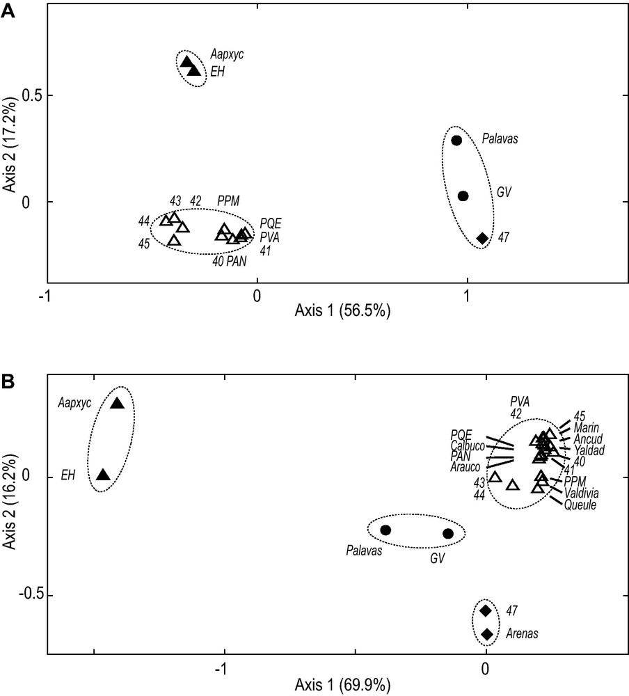
Genetic relationships of Chilean Mytilus spp. Projection of samples from Chile together with reference samples of Northern-Hemisphere Mytilus edulis (EH and Aapxyc), Southern-Hemisphere M. edulis (43–45), Northern-Hemisphere M. galloprovincialis (GV and Palavas), and Southern-Hemisphere M. galloprovincialis (47). Samples were characterized by their electromorph frequencies at allozyme loci and the resulting matrix was subjected to correspondence analysis [35] using the FactoMineR package [36] under R [38]; percentages for each axis are their inertias [35]; ellipses delineate clusters of samples determined by hierarchical clustering [36], allowing the identification to species and subspecies of the tested samples. Full triangles (): Northern-Hemisphere M. edulis; full circles (): Northern-Hemisphere M. galloprovincialis; open triangles (Δ): Southern-Hemisphere M. edulis; diamonds (): Southern-Hemisphere M. galloprovincialis. A. Analysis performed on Matrix-A (15 samples × 8 allozyme loci). B. Analysis performed on Matrix B (23 samples × 2 allozyme loci).
All additional samples from Chile analyzed by [10] but one clustered with the other Chilean samples, together with the Southern-Hemisphere M. edulis samples from the South Atlantic and from the Kerguelen Islands (Fig. 2B). Unlike the Punta Arenas sample of [5], sample ‘Pta. Arenas’ of [10] clustered with the reference sample of Southern-Hemisphere M. galloprovincialis (Fig. 2B).
The nuclear-DNA dataset presented here included two smooth-shelled Mytilus spp. samples from Chile. One sample, from Dichato (CHL), was previously identified as Mediterranean M. galloprovincialis [16]; the other one, from Maullin (MAU), clustered with reference Southern-Hemisphere M. edulis (Fig. 3).
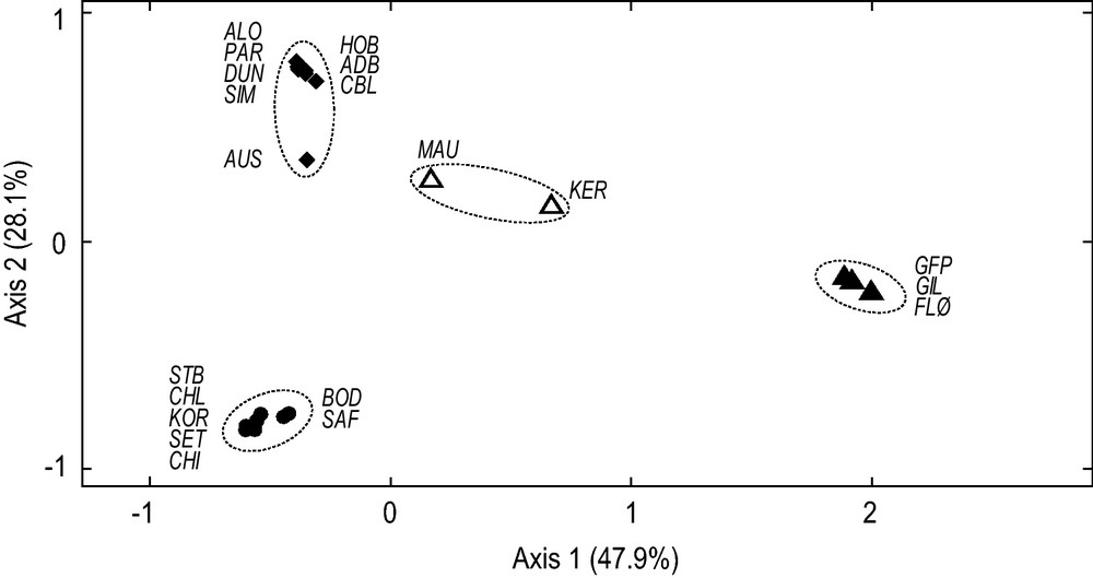
Genetic relationships of Chilean Mytilus spp. Projection of samples from Chile together with reference samples of Northern-Hemisphere Mytilus edulis (FLØ, GFP and GIL), Southern-Hemisphere M. edulis (KER), Northern-Hemisphere M. galloprovincialis (BOD, CHI KOR, SET and STB), and Southern-Hemisphere M. galloprovincialis (ADB, ALO, AUS, CBL, DUN, HOB, PAR and SIM). Samples were characterized by their allelomorph frequencies at nuclear-DNA loci mac-1 and Glu-5′ (Appendix C) and the resulting matrix was subjected to correspondence analysis [35,36]. Ellipses delineate clusters of samples determined by hierarchical clustering [36], allowing the identification to species and subspecies of the tested samples. Full triangles (): Northern-Hemisphere M. edulis; full circles (): Northern-Hemisphere M. galloprovincialis; open triangles (): Southern-Hemisphere M. edulis; diamonds (): Southern-Hemisphere M. galloprovincialis.
Sharp morphological differences were evident between the shells of the two mussel samples from southern central Chile analyzed here (CHL and MAU; Table 2) (Fig. 4). Individuals of the MAU sample clustered with the Southern-Hemisphere M. edulis from Kerguelen whereas those from sample CHL formed a distinct cluster at the center of which the reference sample of Northern-Hemisphere M. galloprovincialis was positioned.
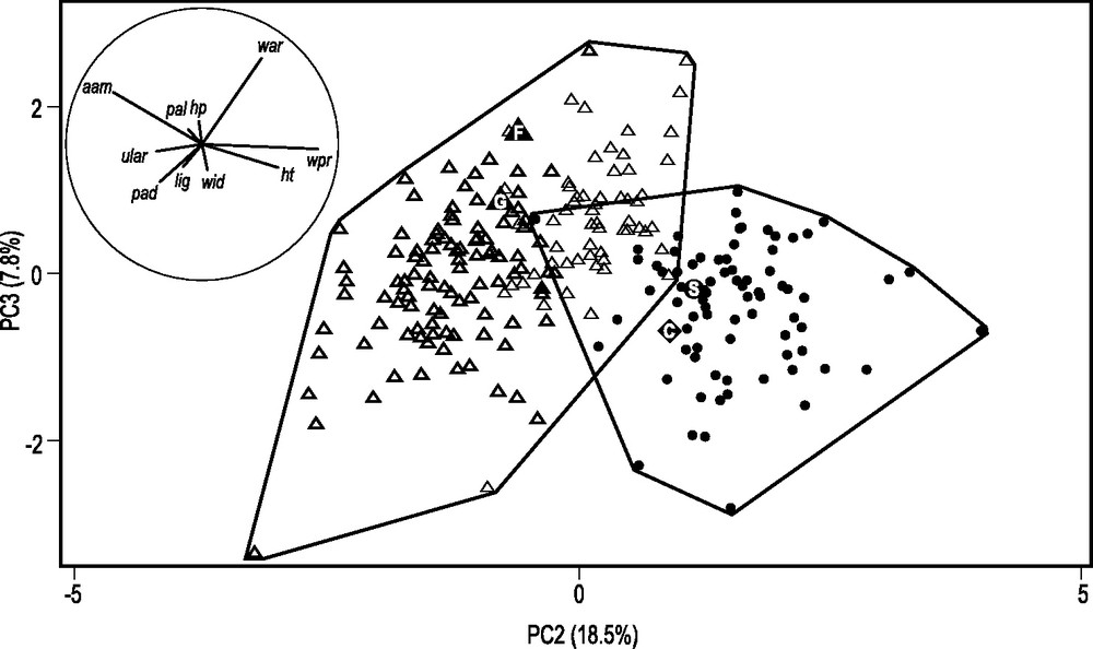
Shell morphometrics of Chilean Mytilus spp. Projection on the plane defined by axes 2 and 3 of principal component analysis (PCA) [37] of individuals sampled in Dichato, Chile (sample CHL in Table 1: full circles; N = 80), Maullin, Chile (MAU: thinner triangles; N = 56) and Kerguelen (KER: thicker triangles; N = 101); insert: correlation circle indicating the relative contribution (proportional to size of arrow) of each shell measurement; the quality of representation of a shell measurement can be visualized by the distance between its projection on the plane and the correlation circle. The left shell of each individual was characterized by 10 measurements according to [5]: length of anterior adductor muscle scar (aam), length of hinge plate (hp), shell height (ht), distance between umbo and posterior end of the ligament (lig), length of posterior adductor muscle scar (pad), distance between pallial line and ventral shell margin midway along shell (pal), distance between umbo and posterior end of anterior retractor scar (ular), width of anterior retractor muscle scar (war), shell width (wid), and width of posterior retractor muscle scar (wpr). Reference Northern-Hemisphere Mytilus edulis (F, G), Northern-Hemisphere M. galloprovincialis (S) and Southern-Hemisphere M. galloprovincialis (C) shells were represented by average values for all 10 measurements in, respectively, samples FLØ (Flødevigen, Skagerrak; N = 53), GIL (Gilleleje, northern Denmark; N = 35), SET (Sète, southern France; N = 55), and CBL (Cloudy Bay Lagoon, Tasmania; N = 96) and incorporated as illustrative variables in the PCA.
4 Discussion
Evidence of alien Mediterranean M. galloprovincialis in Chile so far comes from a single sample, from Dichato (southern central Chile), previously characterized at nuclear-DNA loci mac-1 and Glu-5′ [16] and at the mitochondrial locus COI [21], and here also shown to be morphologically identical to reference Northern-Hemisphere M. galloprovincialis. Additional evidence of Northern-Hemisphere M. galloprovincialis mitotypes has recently been reported in samples from Concepcion and Colchogue, two localities in southern central Chile [18]. All the other smooth-shelled Mytilus samples from Chile reviewed in the present study, but one, were identified as Southern-Hemisphere M. edulis since they clustered with reference samples from the South Atlantic and from the Kerguelen Islands, both genetically and by their shell morphology ([5,21], present study). The exception is a sample from Punta Arenas [10] at the southern tip of South America, which was here identified as Southern-Hemisphere M. galloprovincialis on the basis of allozyme frequencies at loci Pgm and Gpi. This sample has also been analyzed morphologically [11] and found to be significantly different from all the other samples from Chile (distribution of samples along principal component 1 [11]: Dixon's test for detecting outliers [39]; Q = 0.545; N = 8; P < 0.05). The mussels in this sample [10,11] were characterized by a concave and slightly pointed umbo [11], consistent with their allozyme identification as Southern-Hemisphere M. galloprovincialis (present work).
How can we explain the occurrence of Southern-Hemisphere M. galloprovincialis at a location and in a region where only Southern-Hemisphere M. edulis had been previously reported [5]? Southern-Hemisphere M. galloprovincialis are native from temperate Australia, Tasmania, and New Zealand [5,16,18,19,21], while Southern-Hemisphere M. edulis are native from southern South America, the Falkland Islands and the Kerguelen Islands [5,21], and possibly other islands in the Southern Ocean. The distribution areas of the two species are separated by a stretch of ocean of over 105° longitude, from New Zealand to Chile. An hypothesis is that the introduction of Southern-Hemisphere M. galloprovincialis to Punta Arenas is recent and has been caused by maritime traffic, since Punta Arenas is a port of call for global shipping lines that link New Zealand to South America (http://www.timetableimages.com/maritime/). The alternative hypothesis, that both species naturally co-occur in the Punta Arenas area, but that Southern-Hemisphere M. galloprovincialis had previously escaped detection there and all along the cold-temperate shores of South America is, in our view, much less likely. To test the hypothesis that the Southern-Hemisphere M. galloprovincialis sample of [10,11] consists of alien mussels would require genotyping them at marker loci able to distinguish different sub-populations within that population, e.g. the COI marker [21].
Valladares et al. [14] have similarly reported strong morphological differences between cultivated mussels from southern central Chile and wild mussels from the same area and from the Magellanic region of southern Chile. The authors ascribed these differences to differences in ecological pressure on cultivated vs. wild populations. However, no genetic assay was performed, that would help confirm that the cultivated populations analyzed by [14] were native mussels as assumed by the authors, and not alien M. galloprovincialis, despite earlier reports mentioning alien M. galloprovincialis in southern central Chile [16,20,21] and its introduction to mussel farms [20]. Cultivated Chilean mussels differed from wild mussels by umbo shape and orientation, and ligament length [14]. These features have proven useful for distinguishing M. galloprovincialis from M. edulis [5,40]. Therefore, genetic assays are necessary to ascertain that the cultivated smooth-shelled Mytilus samples from southern central Chile analyzed by [14] were not in fact M. galloprovincialis.
In conclusion, the present study confirmed the presence of Mediterranean M. galloprovincialis in southern central Chile, and uncovered the occurrence of Southern-Hemisphere M. galloprovincialis in Punta Arenas. The term ‘M. chilensis’ employed by different authors for smooth-shelled mussels sampled in Chile actually concerns Southern-Hemisphere M. edulis and so-far unreported Southern-Hemisphere M. galloprovincialis, and potentially concerns alien Northern-Hemisphere M. galloprovincialis.
Since morphological characterization of mussel samples has apparently been insufficient for some authors to see mixtures of species in their samples [11], we advocate the systematic use of a genetic assay to identify smooth-shelled Mytilus material from Chile prior to their ecological, physiological or molecular study, or to any related biomonitoring survey. The single marker of choice for identifying smooth-shelled Mytilus spp. to species is mac-1 ([16,22]; present study). In particular, mac-1 allows the distinction of Southern-Hemisphere M. edulis and M. galloprovincialis from their Northern-Hemisphere counterparts [22]. Alternatively, a two-locus diagnostic has been proposed recently [18]. Several studies have employed ITS and Glu-5′ (or Me15/16, which is part of the same gene [34]) to identify Chilean mussels [8,9] but ITS does not separate Southern-Hemisphere M. edulis from either Northern-Hemisphere M. edulis or Northern-Hemisphere M. galloprovincialis [9,41] and Glu-5′ (or Me15/16) does not separate Southern-Hemisphere M. edulis from M. galloprovincialis [18,22,34].
Southern-Hemisphere M. edulis are distinct from Northern-Hemisphere M. edulis at a proportion of nuclear loci ([5,22], present work) and at the mitochondrial locus [21], to an extent that warrants their recognition as a separate, geographically isolated entity. Therefore, it is sensible to assume subspecific rank for them. The valid subspecific name for Southern-Hemisphere M. edulis is M. edulis platensis d’Orbigny 1846 [42] by the principle of priority [43]. Under the same rationale, Southern-Hemisphere M. galloprovincialis should be assigned the subspecific name M. galloprovincialis planulatus Lmk 1819 [2]. Epithet chilensis being a junior synonym of platensis (as is desolationis Lamy 1936 [44]), it should be abandoned.
Disclosure of interest
The authors declare that they have no conflicts of interest concerning this article.
Acknowledgements
The original morphometric and molecular analyses presented in this paper were done at Station méditerranéenne de l’environnement littoral, Sète, in 1997–2000 in the course of CD's Ph.D. and VR's B.Sc. We gratefully acknowledge the support of F. Bonhomme and B. Delay. We are also grateful to J. Beesley, F. Bonhomme, W. Borgeson, P. Boudry, Y. Cherel, P. Fréon, A. Leitao, C. Lemaire, J. Panfili, C. Perrin, and M. Raymond for collecting mussels from, respectively, Nedlands, Chioggia, Bodega Bay, South Korea, Kerguelen, Bloubergstrand, Setubal, Grand Fort Philippe, Flødevigen, Dunedin, and Gilleleje. The mussel sample from Dichato was provided by C. Riquelme and D. Moraga, and that from Maullin was provided by S. Faugeron and S. Morales. We thank D.J. Colgan for editorial corrections on a former version of the manuscript and for encouragements, him and M. Valero for help with the literature, and P. Bouchet and his assistants for curating the mussel specimens deposited by us at MNHN, Paris. J.H. McDonald kindly provided the details in his possession on the sampling sites and dates of reference M. edulis platensis samples. Two anonymous reviewers offered helpful suggestions.
Appendix A
Electromorph frequencies at eight allozyme loci in seven samples of Chilean smooth-shelled mussels (‘Yaldad Bay, Chile’ (40), ‘Chiloe, Chile’ (41), ‘Punta Arenas, Chile’ (42), AN, PPM, PQE and PVA) [5,7] compared with three samples of Southern-Hemisphere Mytilus edulis (‘Mar del Plata, Argentina’ (44), ‘Falkland Islands’ (43) and ‘Kerguelen Islands’ (45)) [5]. Homology of electromorphs between [5] and [26] at loci Ap, Gpi, Lap, Mpi, Odh and Pgm has been established previously [22], and a similar procedure was followed here for locus Aap (‘Lap-1′ of [26]). Homology of electromorphs between [5,26] and [7] were uncovered by comparing samples EH and GV [7] with, respectively, Aapxyc [23] (=’Aarhus, Denmark’ [5]) and Palavas [26] on the basis of relative migrations and similarities in frequencies; when uncertainty about identity remained, electromorphs were pooled as indicated (‘ + ’, ‘≤ ‘, ‘≥’). To complete the Aapxyc sample [23], electromorph frequencies at locus Pgm were taken from the geographically close SWED sample [24]. Sample sizes in brackets.
| Locus, electromorph | Sample | ||||||||||||||||
| [5] | [7] | [26] | 40 | 41 | 42 | 43 | 44 | 45 | 47 | PAN | PVA | PPM | PQE | Aapxyc | EH | Palavas | GV |
| Aap | Lap-1 | Lap-1 | (25) | (23) | (25) | (25) | (25) | (22) | (23) | (41) | (60) | (71) | (71) | (11) | (65) | (93) | (38) |
| ≤ 95 | 93 + 96 | 2 | 0.36 | 0.28 | 0.48 | 0.74 | 0.52 | 0.76 | - | 0.34 | 0.27 | 0.26 | 0.24 | 0.14 | 0.21 | 0.01 | – |
| 100 | 100 | 3 | 0.62 | 0.68 | 0.44 | 0.26 | 0.48 | 0.24 | 0.02 | 0.66 | 0.68 | 0.68 | 0.73 | 0.76 | 0.76 | 0.06 | – |
| 105 | 102 | 4 | 0.02 | 0.02 | 0.04 | – | – | – | – | – | – | 0.02 | 0.01 | 0.10 | 0.01 | 0.09 | – |
| 110 | 104 | 5 | – | 0.02 | 0.04 | – | – | – | 0.15 | – | 0.05 | 0.02 | 0.02 | – | 0.02 | 0.41 | 0.49 |
| 115 + 120 | ≥ 108 | 6 + 7 | – | – | – | – | – | – | 0.83 | – | – | 0.01 | – | – | 0.01 | 0.43 | 0.51 |
| Ap | Ap-1 | Ap | (25) | (23) | (25) | (25) | (25) | (22) | (23) | (41) | (59) | (69) | (72) | (11) | (71) | (92) | (70) |
| 90 + 95 | 93 + 96 | 1 + 2 | – | – | 0.08 | 0.04 | 0.06 | – | – | 0.01 | 0.01 | 0.01 | 0.01 | 0.08 | 0.02 | 0.01 | 0.01 |
| 100 | 100 | 3 | 0.54 | 0.52 | 0.72 | 0.70 | 0.58 | 0.86 | 0.19 | 0.62 | 0.54 | 0.66 | 0.53 | 0.64 | 0.72 | 0.18 | 0.38 |
| 103 | 104 | 4 | – | – | – | – | – | – | – | – | 0.01 | – | – | 0.02 | 0.01 | – | – |
| 105 | 108 | 5 | 0.42 | 0.33 | 0.18 | 0.22 | 0.30 | 0.12 | 0.23 | 0.29 | 0.33 | 0.30 | 0.40 | 0.22 | 0.22 | 0.47 | 0.46 |
| 108 | 114 | 6 | 0.04 | 0.11 | 0.02 | 0.04 | 0.06 | 0.02 | 0.56 | 0.06 | 0.09 | 0.03 | 0.07 | – | 0.04 | 0.16 | 0.13 |
| 117 + 120 | 122 + 128 | 7 + 8 | – | 0.04 | – | – | – | – | 0.02 | 0.01 | 0.02 | 0.01 | – | – | – | 0.18 | 0.03 |
| Est | Est-D | Est-D | (25) | (23) | (25) | (25) | (25) | (22) | (23) | (41) | (61) | (71) | (71) | (11) | (75) | (99) | (72) |
| 80 | 82 | 1.2 | – | – | – | – | – | – | 0.02 | – | – | – | – | – | – | 0.04 | 0.04 |
| 90 | 90 | 4 | 0.30 | 0.59 | 0.08 | – | – | – | 0.48 | 0.62 | 0.57 | 0.45 | 0.63 | 0.04 | 0.01 | 0.94 | 0.91 |
| ≥ 100 | ≥ 100 | ≥ 6 | 0.70 | 0.41 | 0.92 | 1.00 | 1.00 | 1.00 | 0.50 | 0.38 | 0.43 | 0.55 | 0.37 | 0.96 | 0.99 | 0.02 | 0.06 |
| Gpi | Gpi | Pgi | (25) | (23) | (25) | (25) | (25) | (22) | (23) | (41) | (58) | (70) | (69) | (11) | (75) | (94) | (66) |
| ≤ 96 | ≤ 98 | 1 + 2 | – | 0.02 | 0.14 | 0.12 | 0.26 | 0.10 | 0.12 | 0.11 | 0.13 | 0.05 | 0.21 | 0.20 | 0.07 | 0.01 | 0.06 |
| 98 + 100 + 102 | 100 + 102 + 105 | 3 + 4 + 5 | 1.00 | 0.98 | 0.86 | 0.84 | 0.74 | 0.90 | 0.85 | 0.89 | 0.87 | 0.95 | 0.79 | 0.26 | 0.38 | 0.82 | 0.85 |
| ≥ 105 | ≥ 107 | ≥ 6 | – | – | – | 0.04 | – | – | 0.02 | – | – | – | – | 0.54 | 0.55 | 0.18 | 0.09 |
| Lap | Lap-2 | Lap-2 | (25) | (23) | (25) | (25) | (25) | (22) | (23) | (41) | (59) | (71) | (72) | (11) | (72) | (100) | (68) |
| 92 + 94 | 90 + 95 | 1 + 2 | 0.16 | 0.15 | 0.38 | 0.32 | 0.28 | 0.10 | 0.12 | 0.17 | 0.25 | 0.28 | 0.24 | 0.08 | 0.17 | 0.03 | 0.10 |
| 96 | 100 | 3 | 0.82 | 0.81 | 0.62 | 0.68 | 0.72 | 0.90 | 0.79 | 0.82 | 0.75 | 0.68 | 0.73 | 0.70 | 0.58 | 0.46 | 0.54 |
| 98 + 100 | ≥ 102 | 5 + 7 | 0.02 | 0.04 | – | – | – | – | 0.08 | 0.01 | 0.01 | 0.04 | 0.03 | 0.22 | 0.25 | 0.51 | 0.36 |
| Mpi | Mpi | Mpi | (25) | (23) | (25) | (25) | (25) | (22) | (23) | (40) | (59) | (68) | (70) | (11) | (59) | (75) | (56) |
| 90 + 92 | 25 + 100 | 2 | 0.22 | 0.24 | 0.12 | – | 0.06 | 0.02 | 0.96 | 0.26 | 0.36 | 0.16 | 0.4 | 0.06 | 0.02 | 0.97 | 0.97 |
| 96 + 100 | 200 | 3 | 0.78 | 0.76 | 0.88 | 1.00 | 0.88 | 0.98 | 0.04 | 0.73 | 0.64 | 0.84 | 0.6 | 0.94 | 0.98 | 0.03 | 0.03 |
| 110 | 300 | – | – | – | – | – | 0.06 | – | – | 0.01 | – | – | – | – | 0.01 | – | – |
| Odh | Odh | Odh | (25) | (23) | (25) | (25) | (25) | (22) | (23) | (31) | (58) | (68) | (37) | (11) | (64) | (99) | (35) |
| 80 + 90 | 80 + 100 | 1 + 3 | 0.14 | 0.07 | 0.08 | 0.02 | 0.02 | 0.16 | 0.59 | 0.03 | 0.02 | 0.13 | 0.01 | – | 0.06 | 0.15 | 0.49 |
| ≥ 98 | ≥ 112 | ≥ 4 | 0.86 | 0.93 | 0.92 | 0.98 | 0.98 | 0.84 | 0.42 | 0.97 | 0.98 | 0.86 | 0.99 | 1.00 | 0.95 | 0.86 | 0.52 |
| Pgm | Pgm-2 | Pgm | (25) | (23) | (25) | (25) | (25) | (22) | (23) | (37) | (55) | (71) | (72) | (66) | (74) | (96) | (73) |
| ≤ 93 | ≤ 96 | ≤ 3 | 0.02 | – | – | 0.04 | 0.06 | – | 0.29 | 0.03 | – | 0.06 | 0.01 | 0.09 | 0.19 | 0.17 | 0.15 |
| 100 | 100 | 4 | 0.88 | 0.80 | 0.82 | 0.54 | 0.56 | 0.90 | 0.69 | 0.82 | 0.84 | 0.80 | 0.84 | 0.70 | 0.57 | 0.57 | 0.55 |
| ≥ 106 | ≥ 102 | ≥ 6 | 0.10 | 0.20 | 0.18 | 0.42 | 0.38 | 0.10 | 0.02 | 0.15 | 0.16 | 0.15 | 0.15 | 0.21 | 0.24 | 0.27 | 0.30 |
Appendix B
Electromorph frequencies at two allozyme loci in eight samples of Chilean smooth-shelled mussels analyzed by [10]. Homology of electromorphs between [5] and [10] was established as indicated in (“Materials and Methods”). Sample sizes in brackets.
| Locus, electromorph | Sample | ||||||||
| [5] | [10] | Arauco | Queule | Valdivia | Calbuco | Ancud | Yaldad | Marin | Arenas |
| Gpi | GPI | (112) | (80) | (102) | (110) | (110) | (111) | (99) | (107) |
| ≤ 96 | A | 0.11 | 0.03 | 0.03 | 0.10 | 0.10 | 0.07 | 0.13 | 0.13 |
| ≥ 98 | B + C | 0.88 | 0.97 | 0.97 | 0.90 | 0.91 | 0.93 | 0.87 | 0.87 |
| Pgm | PGM | (109) | (108) | (116) | (110) | (99) | (128) | (99) | (100) |
| ≤ 93 | A | 0.03 | 0.07 | 0.06 | 0.02 | 0.01 | 0.01 | 0.01 | 0.30 |
| 100 | B | 0.80 | 0.75 | 0.78 | 0.79 | 0.83 | 0.80 | 0.84 | 0.47 |
| ≥ 106 | C +D | 0.18 | 0.19 | 0.16 | 0.20 | 0.16 | 0.20 | 0.16 | 0.25 |
Appendix C
Allelomorph frequencies at nuclear-DNA loci mac-1and Glu-5’ in 20 samples of smooth-shelled Mytilus spp. including two samples collected in Chile (CHL, MAU). Size homologies between allelomorphs from different samples were ascertained by side-by-side electrophoretic runs. mac-1 allelomorph nomenclature follows [33]; Glu-5′ allelomorphs G, E and E’ [29] are allelomorphs 300, 350 and 380, respectively, in [34]; reference samples from the Northern-Hemisphere (FLØ, GIL, STB, SET, CHI) from [16,22,29,32]. N, sample size.
| Sample | ||||||||||||||||||||
| Locus, Allelomorph | FLØ | GIL | GFP | STB | SET | CHI | SAF | KER | AUS | ADB | ALO | CBL | HOB | PAR | SIM | KOR | DUN | BOD | CHL | MAU |
| mac-1 | ||||||||||||||||||||
| f1 | – | – | – | 0.02 | – | – | 0.02 | – | – | – | – | – | – | – | – | – | – | – | – | – |
| f2 | – | – | – | – | – | – | 0.01 | – | – | – | – | – | – | – | – | – | – | – | – | – |
| f3 | – | – | – | – | – | – | 0.01 | – | – | – | – | – | – | – | – | – | – | – | 0.01 | – |
| b0 | – | – | – | – | – | – | 0.01 | – | – | – | – | – | – | – | – | – | – | – | – | – |
| b05 | – | – | – | – | – | – | – | – | – | – | – | – | – | – | – | – | 0.02 | – | – | – |
| b2 | – | – | – | 0.04 | 0.05 | – | 0.04 | – | – | – | – | – | – | – | – | 0.02 | – | 0.04 | 0.05 | – |
| b1 | – | – | 0.01 | 0.15 | 0.21 | 0.28 | 0.09 | – | 0.04 | – | – | – | – | – | – | 0.42 | – | 0.32 | 0.32 | – |
| b3 | – | – | – | – | – | – | – | – | – | – | – | – | – | – | – | 0.02 | – | – | 0.01 | – |
| b4 | – | – | – | 0.02 | – | 0.01 | – | – | – | – | – | – | – | – | – | – | – | – | – | – |
| b5 | – | – | – | 0.02 | – | – | – | – | – | – | – | – | – | – | – | – | – | – | – | – |
| c1 | – | – | 0.01 | 0.10 | 0.07 | 0.06 | 0.10 | – | – | – | – | – | – | – | – | 0.05 | – | 0.04 | 0.08 | – |
| c12 | – | – | – | – | – | – | – | – | – | – | – | – | – | – | – | – | – | – | 0.01 | – |
| c15 | – | – | – | – | – | – | 0.01 | – | – | – | – | – | – | – | – | – | – | – | – | – |
| c2 | – | – | – | 0.50 | 0.54 | 0.57 | 0.53 | – | 0.16 | – | – | – | – | – | – | 0.43 | – | 0.41 | 0.39 | – |
| c3 | – | – | – | 0.02 | – | 0.01 | 0.04 | – | – | – | – | – | – | – | – | – | – | – | 0.01 | – |
| c4 | 0.05 | – | 0.02 | – | – | – | – | 0.08 | – | – | – | – | – | – | – | – | – | – | – | – |
| c6 | – | – | – | – | 0.01 | – | 0.01 | – | – | – | – | – | – | – | – | – | – | 0.01 | – | – |
| a0 | 0.02 | – | – | – | – | – | – | – | – | – | – | – | – | – | – | – | – | – | – | – |
| a0.5 | – | – | – | – | – | – | – | – | – | – | 0.01 | – | – | – | – | – | 0.04 | – | – | – |
| a1 | 0.06 | 0.02 | 0.01 | 0.02 | – | – | – | – | – | – | – | 0.03 | – | – | – | – | – | – | – | – |
| a15 | – | – | – | – | – | – | – | – | 0.01 | – | – | – | – | – | – | – | 0.01 | – | – | – |
| a2 | 0.10 | 0.15 | 0.20 | 0.02 | – | – | 0.02 | 0.20 | 0.62 | 0.95 | 0.99 | 0.92 | 0.98 | 1.00 | 0.99 | 0.02 | 0.92 | – | 0.03 | 0.26 |
| a3 | 0.29 | 0.31 | 0.24 | 0.04 | 0.01 | – | 0.03 | 0.70 | 0.16 | 0.04 | – | 0.03 | – | – | 0.01 | – | 0.02 | 0.03 | – | 0.74 |
| a4 | 0.07 | 0.17 | 0.18 | – | – | – | – | 0.01 | – | – | – | 0.02 | 0.02 | – | – | – | – | – | 0.01 | – |
| a5 | 0.38 | 0.27 | 0.29 | – | – | – | 0.02 | – | – | – | – | – | – | – | – | – | – | 0.10 | 0.01 | – |
| a6 | – | 0.08 | 0.04 | – | 0.01 | – | 0.02 | – | 0.01 | – | – | – | – | – | – | – | – | – | 0.01 | – |
| a7 | – | – | – | 0.02 | 0.04 | 0.03 | 0.04 | – | – | – | – | – | – | – | – | 0.03 | – | 0.01 | 0.03 | – |
| a8 | – | – | – | 0.04 | 0.06 | 0.03 | 0.01 | – | – | – | – | – | – | – | – | 0.02 | – | 0.01 | 0.05 | – |
| a9 | 0.01 | – | – | – | – | – | – | – | – | – | – | – | – | – | – | – | – | – | – | – |
| d | 0.01 | – | – | – | – | – | – | – | – | – | – | – | – | – | – | – | – | – | – | – |
| (N) | (47) | (26) | (42) | (26) | (68) | (47) | (62) | (83) | (38) | (28) | (59) | (32) | (31) | (30) | (40) | (30) | (79) | (34) | (76) | (51) |
| Glu–5’ | ||||||||||||||||||||
| E +E’ + E” + i | 1.00 | 1.00 | 1.00 | – | 0.01 | – | 0.05 | 0.35 | – | – | – | – | – | – | – | – | – | – | – | – |
| G + i + ii | – | – | – | 1.00 | 0.99 | 1.00 | 0.95 | 0.65 | 1.00 | 1.00 | 1.00 | 1.00 | 1.00 | 1.00 | 1.00 | 1.00 | 1.00 | 0.98 | 1.00 | 1.00 |
| T | – | – | – | – | – | – | – | – | – | – | – | – | – | – | – | – | – | 0.02 | – | – |
| (N) | (35) | (16) | (42) | (19) | (56) | (18) | (65) | (79) | (46) | (26) | (25) | (29) | (26) | (25) | (38) | (19) | (77) | (23) | (48) | (28) |