

1 Introduction
The prey–predator system is an important feature in population dynamics and has been studied by many authors [1–4]. It is already known in the classical predator–prey system where each individual predator possesses the ability to attack prey. Even since research in the discipline of theoretical ecology was initiated by Lotka [5] and Volterra [6], several mathematicians and ecologists contributed to the growth of this area of knowledge and this has been extensively reported in the treatises of Meyer [7], Cushing [8], Conlinvaux [9], Freedman [10], Kapur [11,12]. Recently, the optimal management of renewable resources which has a direct impact on sustainable development, has been studied extensively by Chaudhuri [13], Kar and Swarnakamal [14], and Clark [15]. Now, people are facing the problems due to shortage of resource management. Extensive and unregulated harvesting of marine fish has lead to the extinction of several fish species. These problems are seen in marine reserved zones, where fishing and other activities are prohibited. This marine reserve not only protects species inside the reserve area, but also increases fish abundance in adjacent areas. The model of ecological system reflecting this has been given by Kar and Swarnakamal [14] and Rui Zhang et al. [16]. The ecological interactions are broadly classified as prey-predation, competitions, neutralism, mutualism and so on.
Harvesting has a strong impact on the dynamic evolution of a population. We know, depending on the nature of the applied harvesting strategy, the long-run stationary density of the population may be significantly smaller than the long-run stationary density of a population in the absence of harvesting [15].
Generally, a bionomic model consists of a biological or biophysical type which describes the behaviour of a living system, and an economic model which relates the biological system to market prices and resources with institutional constraints. Bio-economic models contain a single mathematical equation to represent a biological process. The logistic equation is the most commonly used function to capture the essential features of population densities in fishery and forestry management. However, there exists an increasing trend towards simulation models which are developed by biologists and agricultural scientists. These types of models also model the approximate dynamical behaviour in real situations and their complexity may preclude their use directly as part of optimal control models.
As harvesting has a strong impact on the dynamic evolution of a population, depending on the nature of applied harvesting strategy, the long-run stationary density of the population may be significantly smaller than the long-run stationary density of a population in the absence of harvesting. In the absence of harvesting, a population can be free of extinction risk; however, harvesting can lead to the incorporation of a positive extinction probability and to potential extinction in finite time. If a population is subject to a positive extinction rate then harvesting can drive the population density to a dangerous low level at which extinction becomes sure, no matter how the harvester affects the population afterwards. The exploitation of biological resources and harvest of population species are commonly practiced in fishery, forestry and wildlife management. Fishery, an ancient human tradition, has satisfied the food needs of mankind for thousands of years and has become economically, socially and culturally fundamental. Nowadays, fishes are in real trouble as their populations are being depleted to dangerous low levels, and it is necessary to discuss further in order to understand short- and long-term exploitation patterns in fishery management [17].
The problems of predator–prey systems in the presence of harvesting have been discussed by many authors; most of them have focused attention on optimal exploitation guided entirely by profits from harvesting. Brauer and Soudack [18,19] studied a class of predator–prey models under a constant rate of harvesting and under a constant quota of harvesting of both species simultaneously. The prey–predator model with harvesting was also studied by Dai and Tang [20], Myerscough et al. [21], Kar and Chaudhuri [22,23].
Recently, stability analysis of three species with environmental fluctuations was investigated by Gazi et al. [24]. Local stability analysis for a two-species ecological mutualism model has been presented by Reddy et al. [25] and stability analysis of neutral species was carried out by Reddy et al. [26]. Also, the stability analysis of prey, predator and super-predator was carried out by Reddy et al. [2,27]. In 2006, Carletti [28] considered a delay differential equations model with bacteriophage infection and discussed the robustness of the positive equilibrium with respect to stochastic perturbations of the environment using two different approaches. He investigated the analytical estimates of the population intensities with fluctuations by Fourier transform methods. Extensive numerical simulation suggested that a noisy environment for the bacteria population has much more destabilizing behaviour on the concentrations at the equilibrium point than a noisy environment for the phage.
The present investigation is an analytical study of three species system comprising a Prey (S1) common to two predators (S2) and (S3) which are in competition with each other. Some of the equilibrium points are identified based on the model equations and these are given in four distinct classes:
- • in the absence of all species;
- • in the absence of second predator;
- • in the absence of first predator;
- • in the presence of all the species (the co-existent state).
This article is organized in the following way. In the next section, we study the existence of local stability of the equilibria and their dependence on the harvesting efforts. We have concentrated much more on the interior equilibrium of the system as we are interested in the existence of the species. Next, we derived the criteria for the global stabilities of the system. Taking simple economic considerations into account, we have discussed the possibilities of the existence of a bionomic equilibrium when the system is exploited. We also computed the population intensities of fluctuations, i.e., variances around the positive equilibrium due to incorporation of noise which leads to chaos in reality [29]. Some numerical results are presented. The problem ends with a brief description of the principal results obtained here. In particular, our present model could be applied to fish species like goldband fish as a prey, sharks as a first predator and baleen whales or dolphins as second predator in the real ecological arena.
2 Mathematical model
We consider three species multisystem model by the following set of three non-linear ordinary differential equations:
| (1) |
| (2) |
| (3) |
- • xi(t): population density of the species Si at time t; i = 1, 2, 3;
- • ai: the natural growth rates of Si, i = 1, 2, 3;
- • αii: the rate of decrease of Si due to its own insufficient resources, i = 1, 2, 3;
- • α1n: the rate of decrease of the prey due to inhibition by the predators, n = 2, 3;
- • αm1: the rate of increase of the predator due to its successful attacks on the prey, m = 2, 3;
- • Ki = ai/αii: carrying capacities of species, i = 1, 2, 3.
Further, the variables x1, x2 and x3 are non-negative and the model parameters ai, Ki, αij, i = 1, 2, 3, j = 1, 2, 3.
- • q1: catch ability coefficient of prey species;
- • q2: catch ability coefficient of predator species;
- • q3: catch ability coefficient of predator species;
- • E1: effort applied to harvest the prey species (S1);
- • E2: effort applied to harvest the predator species (S2);
- • E3: effort applied to harvest the predator species (S3).
Throughout our analysis, we take the initial conditions as
| (4) |
3 Existence of equilibrium points
The steady state equations of (1)–(3) are
System (1)–(3) possesses the following steady states:
- • the trivial state G1 (0,0,0) (in the absence of all the species);
- • the axial state (in the absence of second predator);
- • the boundary state (in the absence of first predator);
- • the steady state of coexistence G4 (x1*, x2*, x3*) (the interior equilibrium).
Case (i): G1 (0,0,0) i.e. the population is extinct and this state always exists.
Case (ii): if and are the positive solutions of
Then
is positive provided the following inequality holds:
Case (iii): if x1ϕ and x3ϕ are the positive solutions of
Then
x1ϕ is positive provided the following inequality holds:
Case (iv): if x1* and x2* are the positive solutions of
Then
For x1*, x2*, x3* to be positive, the following inequalities hold:
4 Stability
4.1 Local stability analysis
To compute the local stability behaviour, we have studied the variational matrix corresponding to the interior equilibrium. The variational matrix of the system (1)–(3) at G4 (x1*, x2*, x3*) is:
We will point out here that, although (0,0,0) is defined for the system, it cannot be linearised there. So local stability of G1 (0,0,0) cannot be studied. At , the characteristic equation of is since and λ1λ2 = α11α22 + α12α21 > 0. Thus is locally asymptotically stable.
At G3 (x1ϕ, 0, x3ϕ), the characteristic equation of A (x1ϕ, x2ϕ, 0) is , since and λ1λ2 = α11α33 + α31α13 > 0.
Thus G3 (x1ϕ, 0, x3ϕ) is locally asymptotically stable.
The characteristic equation A (x1*, x2*, x3*) is
| (5) |
By the Routh-Hurwitz criterion, it follows that all eigen values of (5) will have negative real parts, if and only if,
Clearly a1 > 0 and a3 > 0, and after some manipulation, it is very easy to check that a1a2 − a3 > 0. Hence G4(x1*, x2*, x3*) is locally asymptotically stable.
4.2 Global stability analysis
In this section, we have considered the global stability of the system (1)–(3) by constructing a suitable Lyapunov function.
Theorem 1. The equilibrium pointis globally asymptotically stable.
Proof: Let us consider the following:
Differentiating V with respect to time t along the solutions of model (1)–(3) and by choosing , a little algebraic manipulation yields
This shows that is negative definite, and hence by the Lyapunov theorem on stability, it follows that the positive equilibrium is globally asymptotically stable with respect to all solutions initiating in the interior of the positive quadrant.
Theorem 2. The equilibrium point G3(x1ϕ, 0, x3ϕ) is globally asymptotically stable.
Proof: Let us consider
This shows that is negative definite, and hence by Lyapunov theorem on stability, it follows that the positive equilibrium G3(x1ϕ, 0, x3ϕ) is globally asymptotically stable with respect to all solutions initiating in the interior of the positive quadrant.
Theorem 3. The equilibrium point G4(x1*, x2*, x3*) is globally asymptotically stable.
Proof: Let us consider
5 Quantitative bionomic aspect of the model
It is mainly associated with study of the dynamics of living resources using economic models. The bionomic equilibrium is said to be achieved when the total revenue obtained by selling the harvested biomass equals the total cost utilized in harvesting. As we have already discussed, a biological equilibrium is given by , i = 1, 2, 3.
Let, c1 be the harvesting cost per unit effort for prey species, c2 be the harvesting cost per unit effort for first predator species (x2), c3 be the harvesting cost per unit effort for the second predator species (x3), p1 be the price per unit biomass of the prey, p2 be the price per unit biomass of the first predator species (x2), p3 be the price per unit biomass of the second predator species (x3).
Therefore, net revenue or economic rent at any time given by R = R1 + R2 + R3 where
The bionomic equilibrium is given by the following equations:
| (6) |
| (7) |
| (8) |
| (9) |
In order to determine the bionomic equilibrium, we come across the following cases.
Case (i): if c1 > p1q1x1, c2 > p2q2x2, c3 > p3q3x3, then the cost is greater than revenue for three species and the whole system will be closed.
Case (ii): if c1 < p1q1x1, c2 < p2q2x2, c3 < p3q3x3, then the revenues for all the species being positive, then the whole system will be in operation.
Now substitute in Eqs. (6)–(9), we get
Now (E1)∞ > 0, if
| (10) |
(E2)∞ > 0, if
| (11) |
| (12) |
Thus the Non-trivial bionomic equilibrium point exists, if conditions (10)–(12) hold.
6 The Stochastic delayed model
Now, we have extended the above model (1)–(3) incorporation the effect of random fluctuations. The sensitive parameters of the system fluctuate about their average values due to these random fluctuations. We incorporated such randomness to the model by adding white noise. The main assumption that leads us to extend the deterministic model (1)–(3) to a stochastic counterpart is that it is reasonable to conceive the open sea as a noisy environment with chaos [30]. There are a number of ways in which environmental noise may be incorporated in system (1)–(3). Generally, the environmental noise is distinguished from demographic or internal noise, for the variation over time is due to different causes. External noise may arise either from random fluctuations of the parameters around some known mean values or from stochastic fluctuations of the population densities around some constant values.
In this section, we computed the population intensities of fluctuations, i.e., variances around the positive equilibrium G4 due to noise, according to the method introduced by Nisbet and Gurney [31]. Now, we assumed the presence of randomly fluctuating driving forces on the deterministic growth of the prey, predator-one and predator-two populations at time t, so that the system (1)–(3) is the following:
| (13) |
| (14) |
| (15) |
| (16) |
| (17) |
Let
| (18) |
| (19) |
Using (18) and (19), Eq. (13) becomes
| (20) |
The linear part of (20) is
| (21) |
Again using (18) and (19), Eq. (14) becomes
| (22) |
The linear part of Eq. (22) is
| (23) |
Using Eqs. (18) and (19), Eq. (15) becomes
| (24) |
The linear part of (24) is
| (25) |
Taking the Fourier transform on both sides of (21), (23), (25) we get:
| (26) |
| (27) |
| (28) |
The matrix form of Eqs. (26)–(28) is
| (29) |
| (30) |
Eq. (29) can also be written as
Let [M(ω)]−1 = K(ω), therefore
| (31) |
| (32) |
| (33) |
If Y has a zero mean value, the inverse transform of SY(ω) is the autocovariance function
| (34) |
The corresponding variance of fluctuations in Y(t) is given by
| (35) |
| (36) |
For a Gaussian white noise process, it is
| (37) |
From (31), we have
| (38) |
From (33) we have
| (39) |
Hence by (35) and (39), the intensities of fluctuations in the variable ui; i = 1, 2, 3 are given by
| (40) |
| (41) |
The real part:
| (42) |
The imaginary part:
| (43) |
Thus Eq. (41) becomes
If we are interested in the dynamics of system (13)–(15) with either η1 = 0 or η2 = 0 or η3 = 0, then the population variances are the following:
(i) if η1 = 0, η2 = 0, then
(ii) if η2 = 0, η3 = 0, then
(iii) if η3 = 0, η1 = 0, then
The expressions in (41) gives three variances of the populations. The integrations over the real line can be evaluated which gives the variances of the populations.
7 Numerical simulation results
In this section, we substantiate as well as augment our analytical findings through numerical simulations considering the following examples.
7.1 Example 1
We take the following parameters:
Fig. 1 shows that the variation of population against time, initially with x1 = 10; x2 = 10; x3 = 20; in three different graphs.
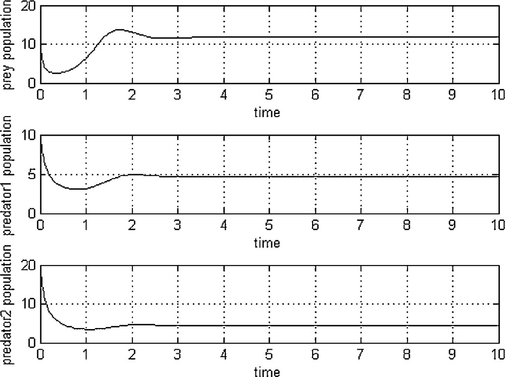
Results of Example 1.
7.2 Example 2
We take the following parameters:
Fig. 2 shows that the variation of population against time, initially with x1 = 10; x2 = 10; x3 = 20; in a single graph.
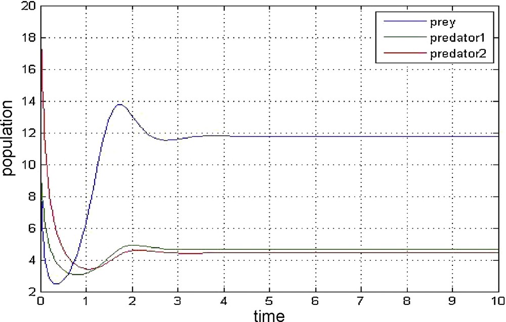
Results of Example 2.
7.3 Example 3
We take the following parameters:
Fig. 3 shows that the variation of population amongst three species prey, predator-one, and predator-two initially with x1 = 10; x2 = 15; x3 = 20; in three dimensions.
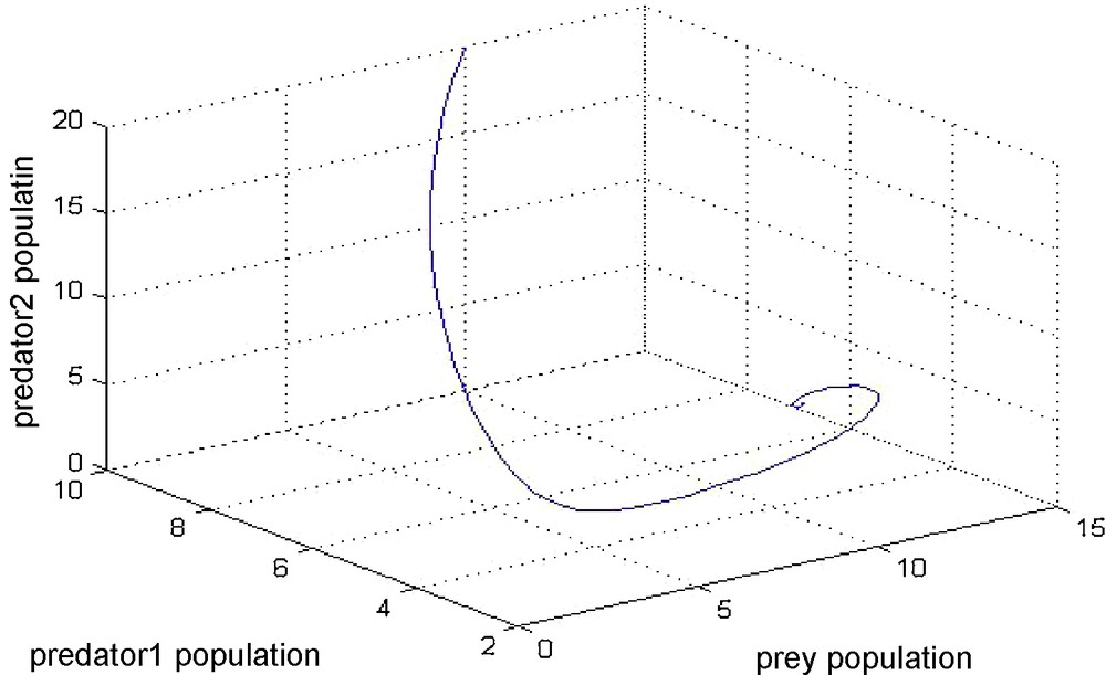
Results of Example 3.
Fig. 4 shows that the population oscillation gives chaos against time under random environmental noise of three species prey, predator-one, and predator-two with initial population sizes x1 = 10; x2 = 15; x3 = 20.
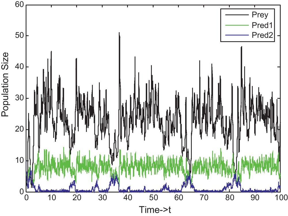
Example 3, population oscillation gives chaos against time.
Fig. 5 shows that the variation of population against time under random environmental noise of species prey, predator-one and predator-two and the fourth is the phase portrait of the same initially with x1 = 10; x2 = 15; x3 = 20.
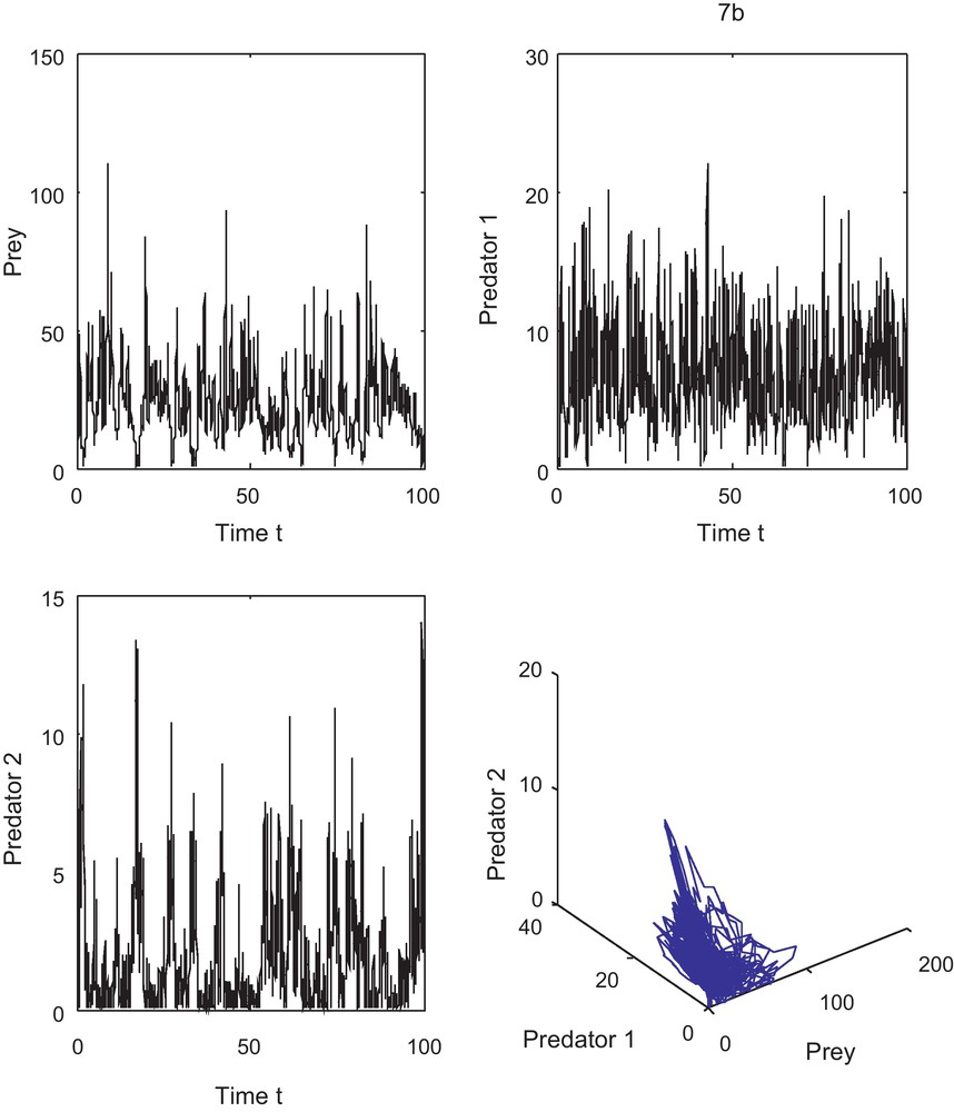
Example 3, variation of population against time under random environmental noise.
8 Concluding remarks
In this article, a mathematical model has been proposed and analysed to study the dynamics of fishery resources. It is assumed that fish populations are growing logistically in reality. Using the stability theory of ordinary differential equations [32], it is known that the interior equilibrium should exist under certain conditions and it is globally asymptotically stable.
From Figs. 1–3, we may conclude that the given biological system is stable and in the case of fish (in particular fish species like goldband fish as a prey, shark as a first predator and baleen whale or dolphin as second predator), Eqs. (10)–(12) are satisfied, then the fishermen will get profit and further, they can run fisheries. Usually fishermen may harvest the predator population to increase profit even though harvesting of predator species is very costly and sometimes difficult [33–35]. However, in the case of prey species fishermen will not get that much profit when compared to predators. Even though, some fishermen will concentrate on the harvesting of prey species, since prey fishes (like goldband small fishes) play a major vital role while curing of the diseases related to eye. Also from the Figs. 4 and 5, we have seen that the system (13)–(15) is chaotic [29,30], in nature as it is a-periodic along with high sensitivity to the initial conditions for solution trajectories in bounded region. Recently, ratio-dependent system interactions have attracted many researchers, as these models produce richer dynamics in real media. The dynamics of ratio-dependent fishery models are also an important area of research which is left for future investigations for good innovative researcher.
Disclosure of interest
The authors declare that they have no conflicts of interest concerning this article.
Acknowledgements
The authors are grateful to the reviewers for their critical evaluations and suggestions.
Appendix A Proof of Theorem 3
Let us consider the Lyapunov function
Choosing , after a little algebraic manipulation, we get,
Now it is very clear that .
Since in some neighbourhood (x1*, x2*, x3*) therefore the interior equilibrium point (x1*, x2*, x3*) is globally asymptotically stable.