Combined harvesting of a stage structured prey–predator model incorporating cannibalism in competitive environment

Kunal Chakraborty; Kunal Das; Tapan Kumar Kar

doi:10.1016/j.crvi.2013.01.002

Population biology/Biologie des populations

Combined harvesting of a stage structured prey–predator model incorporating cannibalism in competitive environment

Kunal Chakraborty ¹ ; Kunal Das ²; Tapan Kumar Kar ³

¹ Information Services and Ocean Sciences Group, Indian National Centre for Ocean Information Services, “Ocean Valley”, Pragathi Nagar (BO), Nizampet (SO), Hyderabad 500090, India
² Department of Mathematics, Sashinara High School, Sashinara, Memari, Burdwan 713146, India
³ Department of Mathematics, Bengal Engineering and Science University, Shibpur, Howrah 711103, India

Comptes Rendus. Biologies, Volume 336 (2013) no. 1, pp. 34-45.

Abstract

In this paper, we propose a prey–predator system with stage structure for predator. The proposed system incorporates cannibalism for predator populations in a competitive environment. The combined fishing effort is considered as control used to harvest the populations. The steady states of the system are determined and the dynamical behavior of the system is discussed. Local stability of the system is analyzed and sufficient conditions are derived for the global stability of the system at the positive equilibrium point. The existence of the Hopf bifurcation phenomenon is examined at the positive equilibrium point of the proposed system. We consider harvesting effort as a control parameter and subsequently, characterize the optimal control parameter in order to formulate the optimal control problem under the dynamic framework towards optimal utilization of the resource. Moreover, the optimal system is solved numerically to investigate the sustainability of the ecosystem using an iterative method with a Runge–Kutta fourth-order scheme. Simulation results show that the optimal control scheme can achieve sustainable ecosystem. Results are analyzed with the help of graphical illustrations.

Supplementary Materials:
Supplementary material for this article is supplied as a separate file:

mmc1.doc

Metadata

Received: 2012-03-09
Accepted: 2013-01-08
Published online: 2013-01-01

PMID

DOI: 10.1016/j.crvi.2013.01.002

Mots-clés : Prey–predator system, Stage structure, Cannibalism, Competitive species, Hopf bifurcation, Global stability, Optimal control

Author's affiliations:

Kunal Chakraborty ¹; Kunal Das ²; Tapan Kumar Kar ³

¹ Information Services and Ocean Sciences Group, Indian National Centre for Ocean Information Services, “Ocean Valley”, Pragathi Nagar (BO), Nizampet (SO), Hyderabad 500090, India
² Department of Mathematics, Sashinara High School, Sashinara, Memari, Burdwan 713146, India
³ Department of Mathematics, Bengal Engineering and Science University, Shibpur, Howrah 711103, India

@article{CRBIOL_2013__336_1_34_0,
     author = {Kunal Chakraborty and Kunal Das and Tapan Kumar Kar},
     title = {Combined harvesting of a stage structured prey{\textendash}predator model incorporating cannibalism in competitive environment},
     journal = {Comptes Rendus. Biologies},
     pages = {34--45},
     publisher = {Elsevier},
     volume = {336},
     number = {1},
     year = {2013},
     doi = {10.1016/j.crvi.2013.01.002},
     language = {en},
}

TY  - JOUR
AU  - Kunal Chakraborty
AU  - Kunal Das
AU  - Tapan Kumar Kar
TI  - Combined harvesting of a stage structured prey–predator model incorporating cannibalism in competitive environment
JO  - Comptes Rendus. Biologies
PY  - 2013
SP  - 34
EP  - 45
VL  - 336
IS  - 1
PB  - Elsevier
DO  - 10.1016/j.crvi.2013.01.002
LA  - en
ID  - CRBIOL_2013__336_1_34_0
ER  -

%0 Journal Article
%A Kunal Chakraborty
%A Kunal Das
%A Tapan Kumar Kar
%T Combined harvesting of a stage structured prey–predator model incorporating cannibalism in competitive environment
%J Comptes Rendus. Biologies
%D 2013
%P 34-45
%V 336
%N 1
%I Elsevier
%R 10.1016/j.crvi.2013.01.002
%G en
%F CRBIOL_2013__336_1_34_0

Kunal Chakraborty; Kunal Das; Tapan Kumar Kar. Combined harvesting of a stage structured prey–predator model incorporating cannibalism in competitive environment. Comptes Rendus. Biologies, Volume 336 (2013) no. 1, pp. 34-45. doi : 10.1016/j.crvi.2013.01.002. https://comptes-rendus.academie-sciences.fr/biologies/articles/10.1016/j.crvi.2013.01.002/

Version originale du texte intégral

1 Introduction

The dynamical analysis of the predator–prey model plays an important role in mathematical biology. Though many biologists believe that if the unique positive equilibrium point of a predator–prey system is locally asymptotically stable, then it is globally asymptotically stable, it is not always true however. It is proved that a unique positive locally asymptotically stable equilibrium point has at least one limit cycle surrounding the equilibrium point under suitable conditions. Thus many mathematicians try to use some well-known methods to find the conditions for global stability for the equilibrium point of predator–prey system [1–8]. Stage-structured population models also have received great attention in recent years. Aiello and Freedman [9] studied a stage-structured model of one species growth consisting of immature and mature members. Cui et al. [10] analyzed the effect of dispersal on the permanence of a stage-structured single-species population model without time delay. A significant amount of research has been carried out based on different kinds of predator–prey systems with division of the predators into immature and mature individuals like Kar and Pahari [11], Magnusson [12], Wang et al. [13], Xu et al. [14], Gao et al. [15], Xu and Ma [16], Chakraborty et al. [17] etc. and references therein.

Ton and Hieu [18] constructed a prey–predator model consisting of one prey and two predators system with Beddington–DeAngelis functional responses. They studied the permanence and extinction of the species and established sufficient conditions for the permanence and extinction. Kar and Chattopadhyay [19] studied the long-run dynamics of a prey–predator model in the presence of an alternative prey. Tian and Xu [20] investigated a stage-structured predator–prey system with Holling type-II functional response. They proved that the predator extinction equilibrium is globally asymptotically stable when the coexistence equilibrium is not feasible and derived sufficient conditions for the global stability of the coexistence equilibrium. Chakraborty et al. [21] described a stage structured prey–predator fishery model where adult prey and predator populations are harvested in the system. They discussed the dynamic behavior of the system and used the fishing effort as a control to develop a dynamic framework to investigate the optimal utilization of the resource. The optimal management of renewable resources as fishery, which has a direct relationship with sustainable development, has been extensively studied by Clark [22,23] and Kot [24] and references therein [25–28].

In the present paper, we have discussed the dynamics of a stage-structured prey–predator fishery system in a competitive environment [29,30]. The asymptotic behavior of the proposed system is analyzed and the sufficient conditions are derived for the global stability of the system at the interior equilibrium point using a geometrical approach. The competitive parameters are used to examine the system transitions at the critical points. Attempt has made to interpret the obtained results in terms of ecology to the extent possible. The control parameter is characterized and the optimal control problem is formulated to it solve using an iterative method with a Runge–Kutta fourth-order scheme. The numerical results provide several realistic features of the model system.

2 Model formulation

We consider a prey–predator model with stage structure for predator and non-selective harvesting is taken into consideration. Let us assume x, y and z are respectively the size of prey population, immature predator population and mature predator population at time t. It is assumed that the populations are growing in a closed homogeneous environment. The growth of prey population is assumed to be logistic and the birth rate of the immature predator population is assumed to be proportional to the density of the existing mature predator population with a proportionality constant β. It is to be noted that cannibalism (which means the act of any population consuming members of its own type or kind, including the consumption of mates) introduces trophic structure and feedback loops within populations. We have assumed the cannibalism or cyclic recruitment pattern of the predator population. In this regard, we have considered that the mature predator population catches the prey population and the immature predator population according to Holling type-II functional response, i.e., respectively, αxz/(a + x) and ωyz/(b + y), where α and ω are the respective maximal predator per capita consumption rate, i.e. the maximum number of prey and immature predator that can be eaten by a predator in each time unit and a, b are the half-capturing saturation constant, i.e. the number of prey and immature predators necessary to achieve one-half of the maximum rates α and ω [31]. It is also assumed that there exist density-dependent factors, competition, between prey population and immature predator population for their survival. The growth of mature predator population is assumed to be of the Leslie-Gower type, with an intrinsic growth rate s and carrying capacity proportional to the sum of the prey and immature predator population size [17,32,33].

In this context, it is to be noted that a study in a Canadian lake showed how the introduced red shiners decreased the rainbow trout population by competition with young trout, even if large trout benefited from the introduction by eating the shiners [34]. Differences in the dynamics, growth, survivorship, and resource use within age classes of interacting populations are often produced by the combined effect of competition and predation [34]. This shows that there is often the need at the present age to study the population dynamics, since very complex interactions work at different levels in populations.

Keeping these aspects in view, the dynamics of the system may be governed by the following system of differential equations:

\begin{array}{l} \frac{d x}{d t} = r x (1 - \frac{x}{K}) - \frac{α x z}{a + x} - σ x y \\ \frac{d y}{d t} = β z - \frac{ω y z}{b + y} - ρ x y \\ \frac{d z}{d t} = s z (1 - \frac{γ z}{x + y}) \end{array}

(2.1)

where r is the intrinsic growth rate of the prey population, K is the environmental carrying capacity of prey population.σ and ρ are the constant coefficients of competition. γ is the equilibrium ratio of predator–prey populations.

Harvesting has a strong impact on the dynamic evaluation of a population subjected to it. First of all, depending on the nature of the applied harvesting strategy, the long-run stationary density of population may be significantly smaller than the long-run stationary density of a population in the absence of harvesting. Therefore, while a population can in the absence of harvesting be free of extinction risk, harvesting can lead to the incorporation of a positive extinction probability and, therefore, to potential extinction in a finite time. Secondly, if a population is subjected to a positive extinction rate, then harvesting can drive the population density to a dangerously low level at which extinction becomes sure, no matter how the harvester affects the population afterwards.

The functional form of the harvest is generally considered using the phrase catch-per-unit-effort (CPUE) hypothesis [23] to describe an assumption that catch per unit effort is proportional to the stock level. Therefore, harvesting function h₁(t), h₂(t) and h₃(t) can be written in the following form:

\begin{array}{l} h_{1} (t) = q_{1} E x, \\ h_{2} (t) = q_{2} E y, \\ h_{3} (t) = q_{3} E z . \end{array}

(2.2)

where q₁, q₂, q₃ are catchability coefficients, E is taken as combined harvesting effort used to harvest the populations.

Finally, using equation (2.2) in (2.1), the system becomes,

\begin{array}{l} \frac{d x}{d t} = r x (1 - \frac{x}{K}) - \frac{α x z}{a + x} - σ x y - q_{1} E x \\ \frac{d y}{d t} = β z - \frac{ω y z}{b + y} - ρ x y - q_{2} E y \\ \frac{d z}{d t} = s z (1 - \frac{γ z}{x + y}) - q_{3} E z \end{array}

(2.3)

with the initial conditions x(0) ≥ 0, y(0) ≥ 0, z(0) ≥ 0.

3 Boundedness of the system

In this section, we intend to establish the conditions to get positive as well as bounded solutions of the system (2.3).

Theorem 3.1

If y(t) is always non-negative, then all possible solutions of the system(2.3)are positive.

Proof

From the first set of equation (2.3) system we can write,

\begin{array}{l} \frac{d x}{d t} = x [(r (1 - \frac{x}{K}) - \frac{α z}{a + x} - q_{1} E - σ y)] \\ \frac{d x}{x} = [(r (1 - \frac{x}{K}) - \frac{α z}{a + x} - q_{1} E - σ y)] d t \\ = ϕ (x, y, z) d t \end{array}

where

ϕ (x, y, z) = [(r (1 - \frac{x}{K}) - \frac{α z}{a + x} - q_{1} E - σ y)]

Taking integration in the region [0,t], we get,

x (t) = x (0) e^{\int ϕ (x, y, z) d t} > 0 \forall t

as x(0) ≥ 0.

Again, from the third equation of the system (2.3) we get,

\begin{array}{l} \frac{d z}{d t} = z [s (1 - \frac{γ z}{x + y}) - q_{3} E] \\ or, \frac{d z}{z} = [s (1 - \frac{γ z}{x + y}) - q_{3} E] d t \\ = ψ (x, y, z) d t \end{array}

where

ψ (x, y, z) = s (1 - \frac{γ z}{x + y}) - q_{3} E

.

By integration in the region [0,t], we get, $z (t) = z (0) e^{\int ψ (x, y, z) d t} > 0 \forall t$ .

Hence, according to our assumption, if we consider $y (t) > 0 \forall t$ , then it may be concluded that all the solutions of the system (2.3) are always positive.

In the remaining part of our analysis, we assume that y(t) is always non-negative, so that the solutions of the system (2.3) are always positive. In the next theorem, we try to find some sufficient conditions for which the solutions of the system (2.3) are bounded.

Theorem 3.2

If E < β/q₂γ, then the solution of the system (2.3) are bounded above.

Proof

From the first equation of the system (2.3), we may conclude that $x (t) < K \forall t$ .

Again, from the third equation of the system (2.3) we may write:

γ z (t) \leq (x (t) + y (t)), \forall t

or, z (t) \leq \frac{(x (t) + y (t))}{γ}, \forall t

Using the above expression in the second equation of the system (2.3), we obtain $\frac{d y}{d t} \leq \frac{β}{γ} (K + y (t)) - q_{2} E$ .

= - (q_{2} E - \frac{β}{γ}) y (t) + \frac{K β}{γ}

= - ξ y + \frac{K β}{γ} where ξ = q_{2} E - \frac{β}{γ}

or \frac{d y}{d t} + ξ y \leq \frac{K β}{γ} .

Now, if $(q_{2} E - \frac{β}{γ}) > 0$ then, ξ > 0 and then, integrating the above equation, we get:

y (t) \leq \frac{ξ y (0) - \frac{K β}{γ}}{ξ - 0} e^{- ξ t} + \frac{K β}{γ} i.e.; y (t) \leq \frac{K β}{γ} \forall t

Thus, we may write $z (t) \leq \frac{(K + \frac{k β}{γ})}{γ} \forall t .$

Hence, all the solutions of the system (2.3) are bounded if $E < \frac{β}{q_{2} γ}$ .

Hence, the theorem is proved.

4 Equilibrium points: existence and stability

To analyze the system (2.3) at its equilibria, we first try to find all possible non-negative equilibria. Clearly, the system has three feasible non-negative equilibria, namely:

• the boundary equilibrium at $P_{1} (\frac{K}{r} (r - q_{1} E),0,0)$ provided $E < \frac{r}{q_{1}}$ ;
• the prey-free equilibria at P₂ (0, y₁, z₁) where $y_{1} = \frac{b [s (q_{2} E - β) + q_{3} E β]}{β s - β q_{3} E - ω s + ω q_{3} E - s q_{2} E}$ and $z_{1} = \frac{b (s - q_{3} E) [s (q_{2} E - β) + q_{3} E β]}{s [(β - ω) (s - q_{3} E) - s q_{2} E]}$ provided β > ω and $\frac{β}{q_{2}} < E < \frac{s}{q_{3}}$ ;
• the interior equilibrium P^*(x^*, y^*, z^*) where (x^*, y^*, z^*) are the positive solution of the system $\dot{x} = \dot{y} = \dot{z} = 0$ .

The third equation of the system (2.3) gives,

z^{*} = \frac{(s - q_{3} E) (x^{*} + y^{*})}{s γ} .

(4.1)

Again, eliminating z^* from the first and third equation of the system (2.3), we get:

A_{1} x^{* 2} + A_{2} x^{*} y^{*} + A_{3} x^{*} + A_{4} y^{*} + A_{5} = 0

where

A_{1} = \frac{r γ s}{K},

A_{2} = - σ γ s, A_{3} = α (s - q_{3} E) + \frac{r γ s a}{K} - (r - q_{1} E), A_{4} = α (s - q_{3} E) + σ γ s, A_{5} = - a γ s (r - q_{1} E)

Consequently, we have y^{*} = - \frac{A_{5} + A_{3} x^{*} + A_{1} x^{* 2}}{A_{2} x^{*} + A_{4}} .

(4.2)

Now eliminating z^* from the second and third equation of the system (2.3), we get

γ s y^{*} (b + y^{*}) (ρ x^{*} + q_{2} E) = (β b + β y^{*} - ω y^{*}) (x^{*} + y^{*}) (s - q_{3} E)

Substituting y^* in the above expression we get,

G_{5} x^{* 5} + G_{4} x^{* 4} + G_{3} x^{* 3} + G_{2} x^{* 2} + G_{1} x^{*} + G_{0} = 0

(4.3)

where,

G_{0} = q_{2} E γ s A_{5} (b A_{4} - A_{5}) - {A_{5}}^{2} (β - ω) (s - q_{3} E) + (s - q_{2} E) β b A_{4} A_{5},

\begin{array}{l} G_{1} = ρ γ s A_{5} (b A_{4} - A_{5}) + q_{2} E γ s (b (A_{2} A_{5} + A_{4} A_{3}) - 2 A_{3} A_{5}) \\ + (s - q_{3} E) (A_{5} A_{2} β b - A_{3} A_{5} (β - ω) - (A_{4} - A_{3}) (β b (A_{4} - A_{5}) + ω A_{5})), \end{array}

\begin{array}{l} G_{2} = ρ γ s (b (A_{2} A_{5} + A_{4} A_{3}) - 2 A_{3} A_{5}) - q_{2} E γ s (A_{1} A_{5} - A_{3} (b A_{2} - {A_{3}}^{2}) + A_{1} (b A_{4} - A_{5})) \\ + (s - q_{3} E) ((A_{1} - A_{2}) (β b A_{4} - A_{5} (β - ω)) - (β - ω) A_{1} A_{5}), \end{array}

\begin{array}{l} G_{3} = - ρ γ s (A_{1} A_{5} - A_{3} (b A_{2} - {A_{3}}^{2}) + A_{1} (b A_{4} - A_{5}) + q_{2} E γ s A_{1} (b A_{2} - 2 A_{3})) \\ + (s - q_{3} E) (A_{1} (β - ω) (A_{4} - A_{3}) - (A_{2} - A_{1}) (β b (A_{2} - (β - ω) A_{5}))), \end{array}

G_{4} = ρ γ s (A_{1} (b A_{2} - 2 A_{3})) - q_{2} E γ s {A_{1}}^{2} + (s - q_{3} E) (β - ω) (A_{2} A_{1} - {A_{1}}^{2}),

G_{5} = - ρ γ s {A_{1}}^{2} .

Therefore, after getting the positive solution of x^* from equation (4.3), it is easy to get the interior positive solution of y^*and z^* from equations (4.1) and (4.2) provided $E < \frac{s}{q_{3}}$ .

Theorem 4.1

The boundary equilibrium $P_{1} (\frac{K}{r} (r - q_{1} E), 0, 0)$ is locally asymptotically stable if the fishing effort used to harvest lies between the biotechnical productivity of the mature predator and the prey population, i.e., $\frac{s}{q_{3}} < E < \frac{r}{q_{1}}$ .

Proof

The characteristic equation of the system (2.3) at $P_{1} (\frac{K}{r} (r - q_{1} E), 0, 0),$ can be written as:

(λ + (r - q_{1} E)) (λ + (ρ \frac{K}{r} (r - q_{1} E) + E q_{2})) (λ - s + q_{3} E) = 0

The roots are $- (r - q_{1} E),$ $- (ρ \frac{K}{r} (r - q_{1} E) + E q_{2})$ and $(s - q_{3} E)$ .

Consequently, $P_{1} (\frac{K}{r} (r - q_{1} E), 0, 0),$ is asymptotically stable if $\frac{s}{q_{3}} < E < \frac{r}{q_{1}}$ .

Theorem 4.2

The prey free equilibrium P₂ (0, y₁, z₁) is unstable if

(s γ + β) < \frac{{y_{1}}^{2} ω}{{(b + y_{1})}^{2}} and E < \frac{s}{q_{3}} .

Proof

The characteristic equation of the system (2.3) at P₂ (0, y₁, z₁) is:

λ (λ^{2} + a_{1} λ + a_{2}) = 0

where

a_{1} = (1 - \frac{q_{3} E}{s}) [(β + γ s) - \frac{{y_{1}}^{2} ω}{{(b + y_{1})}^{2}}],

a_{2} = (\frac{{(s - q_{3} E)}^{2}}{s {(b + y_{1})}^{2}}) [2 {(y_{1} + (b + \frac{ω}{4}))}^{2} - ω (b + \frac{ω}{9})]

Suppose that the three roots are 0, λ₁, λ₂.

Then, $λ_{1} + λ_{2} = - (1 - \frac{q_{3} E}{s}) [(β + γ s) - \frac{{y_{1}}^{2} ω}{{(b + y_{1})}^{2}}]$ and

λ_{1} λ_{2} = (\frac{{(s - q_{3} E)}^{2}}{s {(b + y_{1})}^{2}}) [2 {(y_{1} + (b + \frac{ω}{4}))}^{2} - ω (b + \frac{ω}{9})] .

Therefore, λ₁, λ₂ both are negative if $(s γ + β) < \frac{{y_{1}}^{2} ω}{{(b + y_{1})}^{2}}$ and $E < \frac{s}{q_{3}}$ .

It is to be noted that the saddle-node equilibrium occurs in non-linear systems with one zero eigenvalue when the system undergoes the saddle-node bifurcation, where a saddle and a node approach each other, coalesce into a single equilibrium and then disappear.

It is also evident that saddle-nodes are always unstable.

Now the characteristic equation of the system around its interior equilibrium point P^*(x^*, y^*, z^*) is given by:

λ^{3} + b_{1} λ^{2} + b_{2} λ + b_{3} = 0

(4.4)

where b₁ = c₁–c₂, b₂ = –(x^*y^*ρ)σ – d₁ + d₂, b₃ = –σe₁ – e₂ + e₃,

c_{1} = \frac{r x^{*}}{K} + \frac{s γ z^{*}}{(x^{*} + y^{*})}, c_{2} = \frac{α x^{*} z^{*}}{{(a + x^{*})}^{2}} + \frac{β z^{*}}{y^{*}} + \frac{ω y^{*} z^{*}}{{(b + y^{*})}^{2}},

d_{1} = (\frac{r x^{*} z^{*} β}{K y^{*}}) + (\frac{α s γ x^{*} z^{* 2}}{{(a + x^{*})}^{2} (x^{*} + y^{*})}) + (\frac{β s γ z^{* 2}}{y^{*} (x^{*} + y^{*})}) + (\frac{r x^{*} y^{*} z^{*} ω}{K {(b + y^{*})}^{2}}) + (\frac{ω γ s y^{*} z^{* 2}}{{(b + y^{*})}^{2} (x^{*} + y^{*})}),

\begin{array}{l} d_{2} = + (\frac{α β x^{*} z^{* 2}}{{(a + x^{*})}^{2} y^{*}}) + (\frac{r s γ x^{*} z^{*}}{K (x^{*} + y^{*})}) + (\frac{α s γ x^{*} z^{* 2}}{(a + x^{*}) {(x^{*} + y^{*})}^{2}}) + (\frac{β s γ z^{* 2}}{{(x^{*} + y^{*})}^{2}}) \\ + (\frac{α ω x^{*} y^{*} z^{* 2}}{{(a + x^{*})}^{2} {(b + y^{*})}^{2}}) + (\frac{ω γ s y^{*} z^{* 2}}{(b + y^{*}) {(x^{*} + y^{*})}^{2}}), \end{array}

e_{1} = (\frac{s x^{*} y^{*} z^{*} ρ γ}{(x^{*} + y^{*})}) + (\frac{s x^{*} y^{*} z^{* 2} γ ω}{(b + y^{*}) {(x^{*} + y^{*})}^{2}}),

\begin{array}{l} e_{2} = (\frac{s x^{*} z^{* 3} α β γ}{{(a + x^{*})}^{2} {(x^{*} + y^{*})}^{2}}) + (\frac{s x^{*} z^{* 3} α β γ}{{(a + x^{*})}^{2} y^{*} {(x^{*} + y^{*})}^{2}}) + (\frac{s x^{*} y^{*} z^{* 2} α γ ρ}{{(a + x^{*})}^{2} {(x^{*} + y^{*})}^{2}}) + (\frac{s x^{*} z^{* 2} β γ α}{{(x^{*} + y^{*})}^{2}}) \\ + (\frac{r s x^{*} y^{*} z^{* 2} γ ω}{K {(b + y^{*})}^{2} (x^{*} + y^{*})}) + (\frac{s x^{*} y^{*} z^{* 3} α γ ω}{{(a + x^{*})}^{2} {(b + y^{*})}^{2} {(x^{*} + y^{*})}^{2}}) + (\frac{s x^{*} y^{*} z^{* 3} α γ ω}{{(a + x^{*})}^{2} (b + y^{*}) {(x^{*} + y^{*})}^{2}}), \end{array}

\begin{array}{l} e_{3} = (\frac{r s x^{*} z^{* 2} β γ}{K {(x^{*} + y^{*})}^{2}}) + (\frac{r s x^{*} z^{* 2} β γ}{(x^{*} + y^{*}) K y^{*}}) + (\frac{s x^{*} z^{* 3} α β γ}{{(a + x^{*})}^{2} y^{*} (x^{*} + y^{*})}) + (\frac{r s x^{*} y^{*} z^{* 2} γ ω}{K (b + y^{*}) {(x^{*} + y^{*})}^{2}}) \\ + (\frac{s x^{*} y^{*} z^{* 3} α γ ω}{{(a + x^{*})}^{2} {(b + y^{*})}^{2} (x^{*} + y^{*})}) . \end{array}

It is to be noted that b₁ > 0 if c₁ > c₂. Again, b₃ > 0 if $σ < \frac{e_{3} - e_{2}}{e_{1}}$ .

$Now, b_{1} b_{2} - b_{3} = - σ f_{1} + f_{2}$

where f₁ = (c₁ – c₂) x^*y^*ρ – e₁, f₂ = (c₁ – c₂) (d₂ – d₃) + e₂ – e₃.

It may also be noted that b₃ can be expressed as,

b_{3} = - ρ g_{1} - g_{2} + g_{3}

where

g_{1} = (\frac{s x^{*} y^{*} z^{* 2} α γ}{(a + x^{*}) {(x^{*} + y^{*})}^{2}}) + (\frac{s x^{*} y^{*} z^{*} ρ γ σ}{(x^{*} + y^{*})}),

\begin{array}{l} g_{2} = (\frac{s x^{*} z^{* 3} α β γ}{{(a + x^{*})}^{2} {(x^{*} + y^{*})}^{2}}) + (\frac{s x^{*} z^{* 3} α β γ}{(a + x^{*}) y^{*} {(x^{*} + y^{*})}^{2}}) + (\frac{s x^{*} z^{* 2} β γ α}{(x^{*} + y^{*})}) + (\frac{r s x^{*} y^{*} x^{* 2} γ ω}{K {(b + y^{*})}^{2} (x^{*} + y^{*})}) \\ + (\frac{s x^{*} y^{*} z^{* 3} α γ β}{(a + x^{*}) {(b + y^{*})}^{2} {(x^{*} + y^{*})}^{2}}) + (\frac{s x^{*} y^{*} z^{* 3} α γ ω}{{(a + x^{*})}^{2} (b + y^{*}) {(x^{*} + y^{*})}^{2}}) + (\frac{s x^{*} y^{*} z^{* 2} γ σ ω}{(b + y^{*}) {(x^{*} + y^{*})}^{2}}), \end{array}

\begin{array}{l} g_{3} = (\frac{r s x^{*} z^{*} β γ}{K {(x^{*} y^{*})}^{2}}) + (\frac{r s x^{*} z^{*} β γ}{(x^{*} + y^{*}) K y^{*}}) + (\frac{s x^{*} z^{* 3} α β γ}{{(a + x^{*})}^{2} y^{*} (x^{*} + y^{*})}) + (\frac{r s x^{*} y^{*} z^{* 2} γ ω}{K (b + y^{*}) {(x^{*} + y^{*})}^{2}}) \\ + (\frac{s x^{*} y^{*} z^{*} α γ ω}{{(a + x^{*})}^{2} {(b + y^{*})}^{2} (x^{*} + y^{*})}) . \end{array}

Therefore, b₃ > 0 if $ρ < \frac{g_{3} - g_{2}}{g_{1}}$

$Again, b_{1} b_{2} - b_{3} = - ρ h_{1} + h_{2}$

where h₁ = (c₁ – c₂) x^*y^*σ – g₁, h₂ = (c₁ – c₂) (d₂ – d₃) + g₂ – g₃.

Now, we state and prove the theorem for the local stability of the system around its interior equilibrium point.

Theorem 4.3

The sufficient conditions for the system(2.3)is locally asymptotically stable around its interior equilibrium point P^* (x^*, y^*, z^*) are c₁ > c₂, $σ < \frac{e_{3} - e_{2}}{e_{1}}$ or $(ρ < \frac{g_{3} - g_{2}}{g_{1}})$ and $σ < \frac{f_{2}}{f_{1}}$ or $(ρ < \frac{h_{2}}{h_{1}})$ .

Proof

If the interior equilibrium point P^* (x^*, y^*, z^*) of the system (2.3) exists, then its characteristic equation at the interior equilibrium point is given by equation (4.4).

The condition c₁ > c₂ implies that b₁ > 0.

Again, b₃ > 0 if $σ < \frac{e_{3} - e_{2}}{e_{1}}$ or $(ρ < \frac{g_{3} - g_{2}}{g_{1}})$ .

Finally, $σ < \frac{f_{2}}{f_{1}}$ or $(ρ < \frac{h_{2}}{h_{1}})$ implies that b₁b₂ > b₃.

Hence, by the Routh–Hurwitz criterion, the theorem follows.

5 Bifurcation analysis

We now analyze the bifurcation phenomenon of the proposed system considering competitive parameters, σ and ρ, as the bifurcation parameters. It is easy to show, using Liu's criterion [35], that the system (2.3) undergoes a Hopf bifurcation at its interior equilibrium for the critical value of the competitive parameters σ = σ^* and ρ = ρ^*.

Theorem 5.1

Let us assume that the positive equilibrium is locally asymptotically stable with e₁ > (c₁ – c₂) x^*y^*ρ (or g₁ > (c₁ – c₂) x^*y^*σ); then a simple Hopf bifurcation occurs at the unique real value $σ = σ^{*} = \frac{f_{2}}{f_{1}}$ or $(ρ = ρ^{*} = \frac{h_{2}}{h_{1}})$ .

Proof

The characteristic equation of the model system (2.3) at the interior equilibrium P^* (x^*, y^*, z^*) is given by λ³ + b₁λ² + b₂λ + b₃ = 0.

As it is assumed that the positive equilibrium point P^* (x^*, y^*, z^*) is locally asymptotically stable, therefore it is evident from Theorem 4.4 that b₁ > 0 and b₃ > 0 for all positive values of σ and ρ.

Now, $Δ (σ) = b_{1} (σ) b_{2} (σ) - b_{3} (σ) = - σ f_{1} + f_{2}$

or we can write $Δ (ρ) = b_{1} (ρ) b_{2} (ρ) - b_{3} (ρ) = - ρ h_{1} + h_{2}$ .

Consequently, we have Δ(σ^*) = 0 or Δ(ρ^*) = 0.

Furthermore, ${(\frac{d Δ}{d σ})}_{σ = σ^{*}} = - f_{1} (\neq 0)$ if $e_{1} > (c_{1} - c_{2}) x^{*} y^{*} ρ$ ,

Again, ${(\frac{d Δ}{d ρ})}_{ρ = ρ^{*}} = - h_{1} (\neq 0)$ if $g_{1} > (c_{1} - c_{2}) x^{*} y^{*} σ$ .

Hence, by Liu's criterion, the theorem follows.

6 Global stability

In this section, we will use geometric approach to derive the sufficient conditions for the global stability of the system at the positive equilibrium. For detailed calculations, one can see Chakraborty et al. [17], Li and Muldowney [36], Bunomo et al. [37], Martin [38] etc.

The autonomous system (2.3) can be written as $\frac{d x}{d t} = f (x),$ where

f (x) = (\begin{array}{l} \frac{d x}{d t} = r x (1 - \frac{x}{K}) - \frac{α x z}{a + x} - q_{1} E x - σ x y \\ \frac{d y}{d t} = β z - \frac{ω y z}{b + y} - ρ x y - q_{2} E y \\ \frac{d z}{d t} = s z (1 - \frac{γ z}{x + y}) - q_{3} E z \end{array}), X = (\begin{array}{l} x \\ y \\ z \end{array})

If V(x) be the variation matrix of the system, then it can be written as:

V = \frac{\partial f}{\partial x} = [\begin{array}{c} - \frac{r x}{K} + \frac{α x}{{(a + x)}^{2}} & - σ x & - \frac{α x}{a + x} \\ - ρ y & \frac{β z}{y} + \frac{ω z y}{{(b + y)}^{2}} & - β - \frac{ω y}{b + y} \\ \frac{s γ z^{2}}{{(x + y)}^{2}} & \frac{s γ z^{2}}{{(x + y)}^{2}} & - \frac{s γ z}{x + y} \end{array}]

If $V^{|2|}$ is the second additive compound matrix of V due to Bunomo et al. [37]; we can write:

V^{|2|} = [\begin{array}{c} - \frac{r x}{K} + \frac{α x}{{(a + x)}^{2}} + \frac{β z}{y} + \frac{ω z y}{{(b + y)}^{2}} & - β - \frac{ω y}{b + y} & \frac{α x}{a + x} \\ \frac{s γ z^{2}}{{(x + y)}^{2}} & - \frac{r x}{K} + \frac{α x}{{(a + x)}^{2}} - \frac{s γ z}{x + y} & - σ x \\ - \frac{s γ z^{2}}{{(x + y)}^{2}} & - ρ y & \frac{β z}{y} + \frac{ω z y}{{(b + y)}^{2}} - \frac{s γ z}{x + y} \end{array}]

We consider M(x) in C¹ (D) in a way that $M = diag \{\frac{x}{z}, \frac{x}{z}, \frac{x}{z}\}$ . Then we can write: $M^{- 1} = diag \{\frac{z}{x}, \frac{z}{x}, \frac{z}{x}\}$ and

M_{f} = \frac{d M}{d x} = diag \{\frac{\dot{x}}{z} - (\frac{x}{z^{2}}) \dot{z}, \frac{\dot{x}}{z} - (\frac{x}{z^{2}}) \dot{z}, \frac{\dot{x}}{z} - (\frac{x}{z^{2}}) \dot{z}\}

Thus, easily we can show that,

M_{f} M^{- 1} = diag \{\frac{\dot{x}}{x} - \frac{\dot{z}}{z}, \frac{\dot{x}}{x} - \frac{\dot{z}}{z}, \frac{\dot{x}}{x} - \frac{\dot{z}}{z}\}

and $M V^{|2|} M^{- 1} = V^{|2|}$

So by calculating we get:

B = M_{f} M^{- 1} + M V^{|2|} M^{- 1} = (\begin{array}{c} B_{11} & B_{12} \\ B_{21} & B_{22} \end{array}),

where

B_{11} = (\frac{\dot{x}}{x} - \frac{\dot{z}}{z} - \frac{r x}{K} + \frac{α x z}{{(a + x)}^{2}} - \frac{β z}{y} + \frac{ω y z}{{(b + y)}^{2}})

B_{12} = (\begin{array}{c} - β - \frac{ω y}{b + y} & \frac{α x}{a + x} \end{array})

B_{21} = {(\begin{array}{c} \frac{s γ z^{2}}{{(x + y)}^{2}} & - \frac{s γ z^{2}}{{(x + y)}^{2}} \end{array})}^{t}

B_{22} = (\begin{array}{c} \frac{\dot{x}}{x} - \frac{\dot{z}}{z} - \frac{r x}{K} + \frac{α x z}{{(a + x)}^{2}} - \frac{γ s z}{x + y} & - σ x \\ - ρ y & \frac{\dot{x}}{x} - \frac{\dot{z}}{z} - \frac{β z}{y} + \frac{ω y z}{{(b + y)}^{2}} - \frac{γ s z}{x + y} \end{array})

Now let us define the following vector norm in $R^{3} |< u, v, w >| = \max \{|u|, |v| + |w|\}$ where (u, v, w) is the vector norm in R³ and it is denoted by Γ:

Γ (B) \leq \{p_{1}, p_{2}\}; p_{i} = Γ_{1} (B_{i i}) + |B_{i j}|

Γ_{1} (B_{11}) = \frac{\dot{x}}{x} - \frac{\dot{z}}{z} - \frac{r x}{K} + \frac{α x z}{{(a + x)}^{2}} - \frac{β z}{y} + \frac{ω y z}{{(b + y)}^{2}} .

B_{12} = \max \{|- β - \frac{ω y}{b + y}|, \frac{α x}{a + x}\} .

B_{21} = \max \{\frac{s γ z^{2}}{{(x + y)}^{2}}, - \frac{s γ z^{2}}{{(x + y)}^{2}}\} = |\frac{s γ z^{2}}{{(x + y)}^{2}}| .

Γ_{2} (B_{22}) = \frac{\dot{x}}{x} - \frac{\dot{z}}{z} - \frac{γ s z}{x + y} + \max \{- \frac{r x}{K} + \frac{α x z}{{(a + x)}^{2}}, \frac{β z}{y} + \frac{ω y z}{{(b + y)}^{2}}\}

∴ p_{1} = Γ_{1} (B_{11}) + B_{12}

= \frac{\dot{x}}{x} - \frac{\dot{z}}{z} - \frac{r x}{K} + \frac{α x z}{{(a + x)}^{2}} - \frac{β z}{y} + \frac{ω y z}{{(b + y)}^{2}} + max \{(- β - \frac{ω y}{b + y}), \frac{α x}{a + x}\}

= \frac{\dot{x}}{x} - s (1 - \frac{γ z}{x + y}) + q_{3} E + \frac{α x z}{{(a + x)}^{2}} - \frac{r x}{K} - \frac{β z}{y} + \frac{ω y z}{{(b + y)}^{2}} + \max \{|β + \frac{ω y}{b + y}|, \frac{α x}{a + x}\}

p_{2} = Γ_{2} (B_{22}) + B_{21}

= \frac{\dot{x}}{x} - \frac{\dot{z}}{z} - \frac{γ s z}{x + y} + \max \{- \frac{r x}{K} + \frac{α x z}{{(a + x)}^{2}}, \frac{β z}{y} + \frac{ω y z}{{(b + y)}^{2}}\} + \frac{s γ z^{2}}{{(x + y)}^{2}}

= \frac{\dot{x}}{x} - s + q_{3} E + \frac{s γ z^{2}}{{(x + y)}^{2}} + \max \{- \frac{r x}{K} + \frac{α x z}{{(a + x)}^{2}}, \frac{β z}{y} + \frac{ω y z}{{(b + y)}^{2}}\}

Γ (B) = \frac{\dot{x}}{x} - s + q_{3} E - \min \{\begin{array}{l} \frac{r x}{K} + \frac{β z}{y} - \frac{α x z}{{(a + x)}^{2}} - \frac{ω y z}{{(b + y)}^{2}} - \frac{s γ z}{x + y} - \max \{|β + \frac{ω y}{b + y}|, \frac{α x}{a + x}\}, \\ \{\frac{r x}{K} + \frac{s γ z^{2}}{{(x + y)}^{2}} - \frac{α x z}{{(a + x)}^{2}}, |- \frac{β z}{y} - \frac{ω y z}{{(b + y)}^{2}} + \frac{s γ z}{{(x + y)}^{2}}|\} \end{array}\}

Now we assume that there exists a positive $μ_{1} \in R$ and t₁ > 0 such that:

$μ_{1} = \inf \{x (t), y (t), z (t)\}$ where t > t₁.

Also, we take $μ_{2} = \max \{|β + \frac{ω μ_{1}}{b + μ_{1}}|, \frac{α μ_{1}}{a + μ_{1}}\},$

μ_{3} = \min \{\frac{r μ_{1}}{K} + \frac{β μ_{1}}{μ_{1}} - \frac{α {μ_{1}}^{2}}{{(a + μ_{1})}^{2}} - \frac{ω μ_{1}}{{(b + μ_{1})}^{2}} - \frac{s γ μ_{1}}{2 μ_{1}} - μ_{2}, \frac{r μ_{1}}{K} - \frac{s γ}{4} - \frac{α {μ_{1}}^{2}}{{(a + μ_{1})}^{2}}, |- β - \frac{ω μ_{1}}{{(b + μ_{1})}^{2}} + \frac{s γ}{4}|\}

Then, we can write:

Γ (B) \leq \frac{\dot{x}}{x} - s + q_{3} E - \min \{\begin{array}{l} \frac{r μ_{1}}{K} + β - \frac{α {μ_{1}}^{2}}{{(a + μ_{1})}^{2}} - \frac{ω {μ_{1}}^{2}}{{(b + μ_{1})}^{2}} - \frac{s γ}{2} - μ_{2,} \frac{r μ_{1}}{K} + \frac{s γ}{4} - \frac{α {μ_{1}}^{2}}{{(a + μ_{1})}^{2}} \\ , - β - \frac{ω {μ_{1}}^{2}}{{(b + μ_{1})}^{2}} + \frac{s γ}{4} \end{array}\}

= \frac{\dot{x}}{x} + q_{3} E - s - μ_{3}

i.e., Γ (B) \leq \frac{\dot{x}}{x} - (s - q_{3} E + μ_{3})

i.e., \frac{1}{t} \int_{0}^{t} Γ (B) d s \leq \frac{1}{t} \ln |\frac{x (t)}{x (0)}| - (s - q_{3} E + μ_{3})

\lim_{t \to \infty} \sup \sup \frac{1}{t} \int_{0}^{t} Γ (B (s, x_{0})) d s < - (s - q_{3} E + μ_{3}) < 0

Now, we are asserting the following theorem to the existence of a global stability around its interior equilibrium.

Theorem 6.1

The system(2.1)is globally asymptotically stable around its interior equilibrium if $s + μ_{3} > q_{3} E$ , where:

μ_{3} = \min \{\frac{r μ_{1}}{K} + \frac{β μ_{1}}{μ_{1}} - \frac{α {μ_{1}}^{2}}{{(a + μ_{1})}^{2}} - \frac{ω μ_{1}}{{(b + μ_{1})}^{2}} - \frac{s γ μ_{1}}{2 μ_{1}} - μ_{2}, \frac{r μ_{1}}{K} - \frac{s γ}{4} - \frac{α {μ_{1}}^{2}}{{(a + μ_{1})}^{2}}, |- β - \frac{ω μ_{1}}{{(b + μ_{1})}^{2}} + \frac{s γ}{4}|\}

with $μ_{1} \in R$ such that for t₁ > 0, we have $μ_{1} = \inf \{x (t), y (t), z (t)\}$ whenever t > t₁.

7 Optimal control problem

In commercial exploitation of renewable resources, the fundamental problem from the economic point of view is to determine the optimal trade off between present and future harvests. The emphasis of this section is on the profit making aspect of fisheries. It is an elaborate study of the optimal harvesting policy and the profit earned by harvesting, focusing on the quadratic cost and conservation of fish population by constraining the letter to always study above a critical threshold. The main reasoning for the quadratic cost is that it allows us to derive an analytical expression for the optimal harvest; the resulting solution is different from the bang-bang solution, which is usually obtained in the case of a linear cost function.

In this section, our objective is to optimize (maximize) the total discount net revenue earned from the fishery. Symbolically, our strategy is to maximize the present value J, which is to be formulated as:

J (E) = \int_{t_{0}}^{t_{f}} e^{- δ t} [(p_{1} - v_{1} q_{1} E x) q_{1} E x + (p_{2} - v_{2} q_{2} E y) q_{2} E y + (p_{3} - v_{3} q_{3} E z) q_{3} E z - c E] d t

(8.1)

where v_t,i = 1, 2, 3 are the economic constants and δ is the instantaneous annual discount rate. c is the constant fishing cost per unit effort, p_i,i = 1, 2, 3 are the constant price per unit biomass of landed fish respectively for prey, immature and mature predator populations.

The problem subjected to the population equation (2.3) and control constraints $0 \leq E \leq E_{Max},$ can be solved by Pointagrin's Maximum Principle.

The convexity of the objective function with respect to E, the linearity of the differential equations in the control and the compactness of the range values of the state variables can be combined to give the existence of the optimal control.

Suppose E_δ is an optimal control with the corresponding states x_δ, y_δ and z_δ. We are seeking to derive the optimal control E_δ such that:

J (E_{δ}) = \max \{J (E) : E \in U\},

where U is the control set defined by:

U = {E : [t_{0}, t_{f}] \to [0, E_{\max}] | E is Lebesgue measurable} .

The Hamiltonian of this control problem is:

\begin{array}{l} H = [(p_{1} - v_{1} q_{1} E x) q_{1} E x + (p_{2} - v_{2} q_{2} E y) q_{2} E y + (p_{3} - v_{3} q_{3} E z) q_{3} E z - c E] + λ_{1} [r x (1 - \frac{x}{K}) \\ - \frac{α x z}{a + x} - q_{1} E x - σ x y] + λ_{2} [β z - \frac{ω y z}{b + y} - ρ x y - q_{2} E y] + λ_{3} [s z (1 - \frac{γ z}{x + y}) - q_{3} E z] \end{array}

where λ₁(t), λ₂(t) and λ₃(t) are the adjacent variables.

The transversality conditions give λ_i(t_f) = 0, i = 1, 2, 3.

Now, it is possible to find the characterization of the optimal control E_δ.

On the set ${t | 0 < E_{δ} (t) < E_{\max}}$ , we have:

\frac{\partial H}{\partial E} = x (- λ_{1} + p_{1}) q_{1} + y (- λ_{2} + p_{2}) q_{2} + z (- λ_{3} + p_{3}) q_{3} - 2 E (x^{2} {q_{1}}^{2} v_{1} + y^{2} {q_{2}}^{2} v_{2} + z^{2} {q_{3}}^{2} v_{3}) - c = 0

at E_δ(t).

This implies that:

E_{δ} = \frac{x_{δ} p_{1} q_{1} + y_{δ} p_{2} q_{2} + z_{δ} p_{3} q_{3} - x_{δ} λ_{1} q_{1} - y_{δ} λ_{2} q_{2} - z_{δ} λ_{3} q_{3} - c}{2 ({x_{δ}}^{2} {q_{1}}^{2} v_{1} + {y_{δ}}^{2} {q_{2}}^{2} v_{2} + {z_{δ}}^{2} {q_{3}}^{2} v_{3})} .

(8.2)

Now, the adjacent equations are

\begin{array}{l} \frac{d λ_{1}}{d t} = δ λ_{1} - \frac{\partial H}{\partial x} = δ λ_{1} - [r (1 - \frac{2 x}{K}) - \frac{α z}{a + x} + \frac{α x z}{{(a + x)}^{2}} - q_{1} E - σ y] λ_{1} + ρ y λ_{2} \\ - \frac{γ z}{{(x + y)}^{2}} λ_{3} - (p_{1} - 2 v_{1} q_{1} E x) q_{1} E x, \end{array}

(8.3)

\frac{d λ_{2}}{d t} = δ λ_{2} - \frac{\partial H}{\partial y} = δ λ_{2} + λ_{1} σ x + [\frac{ω z}{b + y} - \frac{ω y z}{{(b + y)}^{2}} + ρ x + q_{2} E] λ_{2} + \frac{s γ z^{2}}{{(x + y)}^{2}} λ_{3},

(8.4)

\frac{d λ_{3}}{d t} = δ λ_{3} - \frac{\partial H}{\partial z} = δ λ_{3} + \frac{α x}{a + x} λ_{1} - λ_{2} β + \frac{ω z}{b + y} λ_{2} - [s (1 - \frac{2 γ z}{x + y}) - q_{3}] λ_{3} .

(8.5)

Therefore, we summarize the above analysis by the following theorem:

Theorem 8.1

There exist an optimal control E_δand corresponding solutions x_δ, y_δand z_δand that maximizes J(E) over U. Furthermore, there exists adjoint functions λ₁, λ₂and λ₃satisfying equations(8.3)–(8.5) with transversality conditions λ_i(t_f) = 0, i = 1, 2, 3. Moreover, the optimal control is given by:

E_{δ} = \frac{x_{δ} p_{1} q_{1} + y_{δ} p_{2} q_{2} + z_{δ} p_{3} q_{3} - x_{δ} λ_{1} q_{1} - y_{δ} λ_{2} q_{2} - z_{δ} λ_{3} q_{3} - c}{2 ({x_{δ}}^{2} {q_{1}}^{2} v_{1} + {y_{δ}}^{2} {q_{2}}^{2} v_{2} + {z_{δ}}^{2} {q_{3}}^{2} v_{3})} .

8 Numerical simulation

As the problem is not a case study, the real world data are not available for this model. We, therefore, take here some hypothetical data with the sole purpose of illustrating the analytical results that we have established in the previous sections. Moreover, it may be noted that as the parameters of the model are not based on real world observations, the main features described by the simulations presented in this section should be considered from a qualitative, rather than a quantitative point of view. However, numerous scenarios covering the breadth of the biological feasible parameter space were conducted and the results shown above display the gamut of dynamical results collected from all the scenarios tested.

8.1 Numerical simulation to study the bifurcation phenomenon

In order to ensure the existence of bifurcation, let us consider the following parameter set:

\begin{array}{l} r = 1.5, K = 100, α = 0.5, a = 5, q_{1} = 0.5, q_{2} = 0.8, q_{3} = 0.2, b = 2.0, ω = 0.5, γ = 0.6, ρ = 0.08 \\ β = 0.4, s = 0.5, E = 0.2 \end{array}

It is to be noted that if we consider the value of, ρ = 0.13591, then it is observed from Fig. 1 that P^*(x^*, y^*, z^*) is locally asymptotically stable and the populations x, y and z converge to their steady states in finite time. Now if we gradually increase the value of ρ, keeping other parameters fixed, then by Theorem 5.1, it is easy to get a critical value of ρ as ρ^* = 0.14591 such that P^*(x^*, y^*, z^*) loses its stability as ρ passes through ρ^*. Figs. 2 and 3 clearly show the result. It may also be noted that if we consider the value of ρ = 0.15591, then it is evident from Fig. 4 that the positive equilibrium P^*(x^*, y^*, z^*) is unstable. Moreover, a periodic orbit may be observed near P^*(x^*, y^*, z^*).

Fig. 1
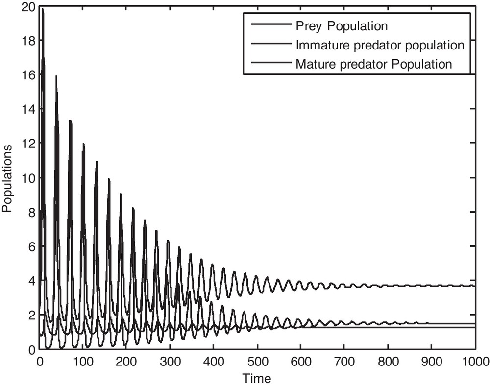
Solution curves of the prey population, immature predator population and mature predator population as a function of time when ρ = 0.13591.

Fig. 2
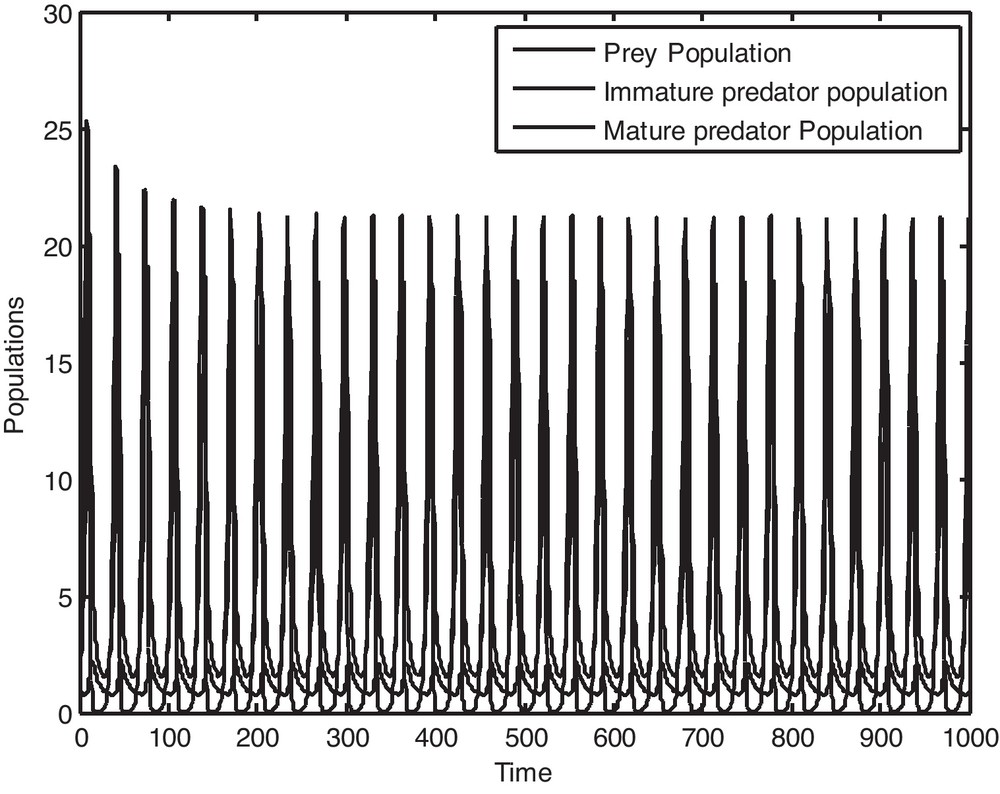
Solution curves of the prey population, immature predator population and mature predator population as a function of time when ρ = 0.14591.

Fig. 3
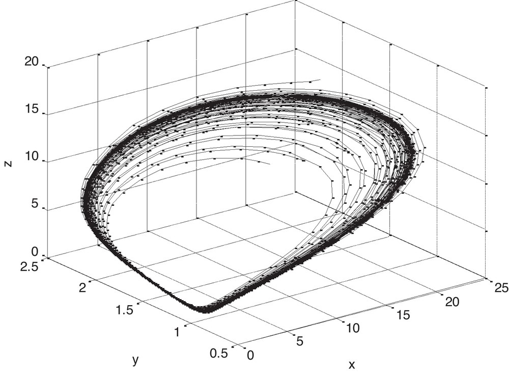
Phase plane trajectories of different biomasses with the different initial levels when ρ = 0.14591.

Fig. 4
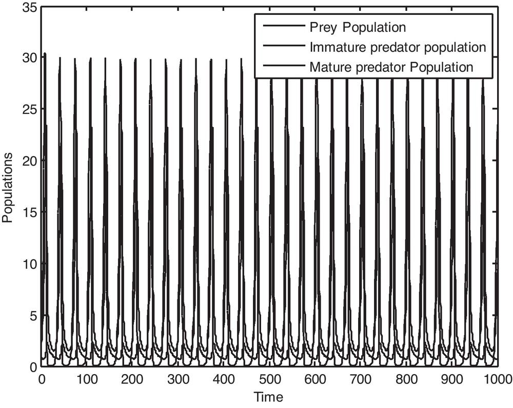
Solution curves of the prey population, immature predator population and mature predator population as a function of time when ρ = 0.15591.

8.2 Numerical simulation to study the optimal control problem

The numerical simulation of optimal control [39] under various parameters set can be done using the fourth-order Runge–Kutta forward-backward sweep method; the system state equations (2.3) and their corresponding adjoint equations (8.3)–(8.5) are simultaneously solved. Initially, we make a guess for optimal control and then solved the system of state equations (2.3) forward in time using the Runge–Kutta method with the initial conditions x₀, y₀ and z₀. Then, using state values, the adjoined equations (8.3)–(8.5) are solved backward in time using the Runge–Kutta method with the transversality condition. At this point, the optimal control is updated using the values for the state and adjoint variables. The updated control replaces the initial control and the process is repeated until the successive iterations of the control values are sufficiently close. The convergence of such an iterative method is based on work of Hackbush [40].

At first, we discretize the interval [t₀, t_n] at the points $t_{i} = t_{0} + i h (i = 0, 1, 2,..., n)$ where h is the time step such that t_n = t_f. Now a combination of forward and backward difference approximation is considered to solve the system. The time derivative of state variables can be expressed by their first-order forward difference as follows:

\frac{x_{i + 1} - x_{i}}{h} = r x_{i + 1} (1 - \frac{x_{i + 1}}{K}) - \frac{α x_{i + 1} z_{i}}{a + x_{i + 1}} - q_{1} E x_{i + 1} - σ x_{i + 1} y_{i},

\frac{y_{i + 1} - y_{i}}{h} = β z_{i} - \frac{ω z_{i} y_{i + 1}}{b + y_{i + 1}} - δ x_{i + 1} y_{i + 1} - q_{2} E y_{i + 1},

\frac{z_{i + 1} - z_{i}}{h} = s z_{i + 1} (1 - \frac{γ z_{i + 1}}{x_{i + 1} + y_{i + 1}}) - q_{3} E z_{i + 1} .

By using a similar technique, we approximate the time derivative of the adjoint variables by their first-order backward difference and we use the approximate scheme as follows:

\begin{array}{l} \frac{{λ_{1}}^{n - i} - {λ_{1}}^{n - i - 1}}{h} = δ {λ_{1}}^{n - i - 1} - [r (1 - \frac{2 x_{i + 1}}{K}) - \frac{α z_{i + 1}}{a + x_{i + 1}} + \frac{α x_{i + 1} z_{i + 1}}{{(a + x_{i + 1})}^{2}} - q_{1} E - σ y_{i + 1}] {λ_{1}}^{n - i - 1} \\ + ρ y_{i + 1} {λ_{2}}^{n - i} - \frac{γ z_{i + 1}}{{(x_{i + 1} + y_{i + 1})}^{2}} {λ_{3}}^{n - i} - (p_{1} - 2 v_{1} q_{1} E x_{i + 1}) q_{1} E x_{i + 1}, \end{array}

\begin{array}{l} \frac{{λ_{2}}^{n - i} - {λ_{2}}^{n - i - 1}}{h} = δ {λ_{2}}^{n - i - 1} + {λ_{1}}^{n - i - 1} σ x_{i + 1} + [\frac{ω z_{i + 1}}{b + y_{i + 1}} - \frac{ω y_{i + 1} z_{i + 1}}{{(b + y_{i + 1})}^{2}} + ρ x_{i + 1} + q_{2} E] {λ_{2}}^{n - i - 1} \\ + \frac{s γ {z_{i + 1}}^{2}}{{(x_{i + 1} + y_{i + 1})}^{2}} {λ_{3}}^{n - i - 1} - (p_{2} - 2 v_{2} q_{2} E y_{i + 1}) q_{2} E y_{i + 1}, \end{array}

\begin{array}{l} \frac{{λ_{3}}^{n - i} - {λ_{3}}^{n - i - 1}}{h} = δ {λ_{3}}^{n - i - 1} + \frac{α x_{i + 1}}{a + x_{i + 1}} {λ_{1}}^{n - i - 1} - {λ_{2}}^{n - i - 1} β + \frac{ω z_{i + 1}}{b + y_{i + 1}} {λ_{2}}^{n - i - 1} \\ - [s (1 - \frac{2 γ z_{i + 1}}{x_{i + 1} + y_{i + 1}}) - q_{3}] {λ_{3}}^{n - i - 1} - (p_{3} - 2 v_{3} q_{3} E z_{i + 1}) q_{2} E z_{i + 1} . \end{array}

The sensitivity of the biological as well as economic parameters of the system on the optimal prey population, immature and mature predator population and also on the fishing effort can be studied using the numerical solution of the optimal control problem.

9 Conclusion

This paper deals with a prey–predator type fishery system which incorporates cannibalism in competitive environment with stage structured for the predator. The interactions among immature and mature species are based on the assumptions as follows: (i) the recruitment of the immature species depend on the size of the mature species; (ii) two substocks interact via cannibalism; (iii) immature predator population which are the product of the mature predator also become mature and (iv) prey population and immature predator population compete with each other for their survival. Though our paper is not based on a case study, Canadian lake fishery may be a good example for our model as red shiners population of Canadian lake fishery decreased the rainbow trout population by competition with young trout, even if large trout benefited from the introduction by eating the shiners.

The dynamics of the proposed system is analyzed in the presence of combined harvesting. Though cannibalism plays an important role towards achieving a sustainable ecosystem, however, it may be noted that so far very few research articles incorporate the effects of cannibalism in the growth of a species in a prey–predator system. It is evident from our study that the cannibalism can be considered as an important structural force in population dynamics. Moreover, our results depict that cannibalism can be considered as an essential biotic process for the populations life in environments characterized by large fluctuations in food resources. The cannibalism in the predator population creates different behavior in the the prey–predator system and thus alters the impact of a predator on prey population dynamics. It may also be concluded that cannibalism decreases the probability of extinction of the species of an ecosystem.

It is observed that for the boundedness of the system, it is necessary to control the fishing effort used to harvest the populations. The criterion for the existence of several equilibria, stabilities and bifurcations of the system are derived. It is further noted that the saddle-node equilibrium occurs to the non-linear systems at the prey free equilibrium. Our results suggest that the density-dependent competitive coefficients may lead a stable equilibrium to become unstable through a simple Hopf bifurcation as the density-dependent competitive coefficients for the species passes through its critical value. It is also clear that when density-dependent competitive coefficients for the species are large, both prey and predator populations reach periodic oscillations around the equilibrium in finite time then converge to their equilibrium values. However, as the density-dependent competitive coefficients for the species decreases, oscillations also increase and the positive steady state disappears; then the consumer population dies out.

It may also be pointed out that in this paper, several important parameters such as ecological fluctuations, refuge, interaction with other species etc. are disregarded. Hence, further research is necessary to accomplish the needs in this field.

Disclosure of interest

The authors declare that they have no conflicts of interest concerning this article.

Acknowledgement

We are very grateful to the anonymous reviewers for their careful reading, constructive comments and helpful suggestions, which have helped us to improve the presentation of this work significantly. The first author also gratefully acknowledges the director of INCOIS for his encouragements and unconditional help. This is INCOIS contribution number 131.

References

[1] G. Dai; M. Tang Coexistence region and global dynamics of a harvested predator–prey system, SIAM J. Appl. Math., Volume 58 (1998), pp. 193-210

[2] T.K. Kar; A. Batabyal Stability and bifurcation of a prey–predator model with time delay, C. R. Biologies, Volume 332 (2009) no. 7, pp. 642-651

[3] M.R. Myerscough; B.F. Gray; W.L. Hogarth; J. Norbury An analysis of an ordinary differential equation model for a two-species predator–prey system with harvesting and stocking, J. Math. Biol., Volume 30 (1992), pp. 389-411

[4] D. Xiao; S. Ruan Bogdanov–Takens bifurcations in predator–prey systems with constant rate harvesting, Fields Inst. Commun., Volume 21 (1999), pp. 493-506

[5] R. Mchich; P. Auger; N. Raïssi The stabilizability of a controlled system describing the dynamics of a fishery, C. R. Biologies, Volume 328 (2005) no. 4, pp. 337-350

[6] T.K. Kar; K. Chakraborty Bioeconomic modelling of a prey–predator system using differential algebraic equations, Int. J. Eng. Sci. Technol., Volume 2 (2010) no. 1, pp. 3-34

[7] T.K. Kar; H. Matsuda Global dynamics and controllability of a harvested prey–predator system with Holling type III functional response, Nonlinear Anal. Hybrid Syst., Volume 1 (2007), pp. 59-67

[8] L. Chen; F. Chen Global analysis of a harvested predator–prey model incorporating a constant prey refuge, Int. J. Biomath., Volume 3 (2010) no. 2, pp. 205-223

[9] W.G. Aiello; H.I. Freedman A time-delay model of single-species growth with stage structure, Math. Biosci., Volume 101 (1990), pp. 139-153

[10] J. Cui; L. Chen; W. Wang The effect of dispersal on population growth with stage-structure, Comput. Math. Appl., Volume 39 (2000), pp. 91-102

[11] T.K. Kar; U.K. Pahari Modelling and analysis of a prey–predator system with stage-structure and harvesting, Nonlinear Anal. Real World Appl., Volume 8 (2007), pp. 601-609

[12] K.G. Magnusson Destabilizing effect of cannibalism on a structured predator prey system, Math. Biosci., Volume 155 (1999), pp. 61-75

[13] W. Wang; G. Mulone; F. Salemi; V. Salone Permanence and stability of a stage-structured predator prey model, J. Math. Anal. Appl., Volume 262 (2001), pp. 499-528

[14] R. Xu; M.A.J. Chaplain; F.A. Davidson Global stability of a Lotka Volterra type predator prey model with stage structure and time delay, Appl. Math. Comput., Volume 159 (2004), pp. 863-880

[15] S. Gao; L. Chen; Z. Teng Hopf bifurcation and global stability for a delayed predator prey system with stage structure for predator, Appl. Math. Comput., Volume 202 (2008), pp. 721-729

[16] R. Xu; Z. Ma Stability and Hopf bifurcation in a ratio-dependent predator prey system with stage structure, Chaos Solut. Fract., Volume 38 (2008), pp. 669-684

[17] K. Chakraborty; S. Jana; T.K. Kar Global dynamics and bifurcation in a stage structured prey–predator fishery model with harvesting, Appl. Math. Comput., Volume 218 (2012) no. 18, pp. 9271-9290

[18] T.V. Ton; N.T. Hieu Dynamics of species in a model with two predators and one prey, Nonlinear Anal. Theory Methods Appl., Volume 74 (2011) no. 14, pp. 4868-4881

[19] T.K. Kar; S.K. Chattopadhyay A focus on long-run sustainability of a harvested prey–predator system in the presence of alternative prey, C. R. Biologies, Volume 333 (2010) no. 11–12, pp. 841-849

[20] X. Tian; R. Xu Global dynamics of a predator–prey system with Holling type II functional response, Nonlinear Anal. Model. Control, Volume 16 (2011) no. 2, pp. 242-253

[21] K. Chakraborty; S. Das; T.K. Kar Optimal control of effort of a stage structured prey–predator fishery model with harvesting, Nonlinear Anal. Real World Appl., Volume 12 (2011) no. 6, pp. 3452-3467

[22] C.W. Clark Bioeconomic Modelling and Fisheries Management, Wiley Series, New York, 1985

[23] C.W. Clark Mathematical Bioeconomics: The Optimal Management of Renewable Resources, Wiley Series, New York, 1990

[24] M. Kot Elements of Mathematical Ecology, Cambridge University Press, Cambridge, UK, 2001

[25] Z. Ge; J. Yan Hopf bifurcation of a predator–prey system with stage structure and harvesting, Nonlinear Anal. Theory Methods Appl., Volume 74 (2011) no. 2, pp. 652-660

[26] L. Chen; F. Chen; L. Chen Qualitative analysis of a predator–prey model with Holling type II functional response incorporating a constant prey refuge, Nonlinear Anal. Real World Appl., Volume 11 (2010) no. 1, pp. 246-252

[27] Q. Gan; R. Xu; P. Yang Bifurcation and chaos in a ratio-dependent predator–prey system with time delay, Chaos Solut. Fract., Volume 39 (2009) no. 4, pp. 1883-1895

[28] X. Zhang; Q.L. Zhang Bifurcation analysis and control of a class of hybrid biological economic models, Nonlinear Anal. Hybrid Syst., Volume 3 (2009) no. 4, pp. 578-587

[29] S. Ruan; A. Ardito; P. Ricciardi; D.L. DeAngelis Coexistence in competition models with density-dependent mortality, C. R. Biologies, Volume 330 (2007) no. 12, pp. 845-854

[30] R. Arditi; J. Callois; Y. Tyutyunov; C. Jost Does mutual interference always stabilize predator–prey dynamics? A comparison of models, C. R. Biologies, Volume 327 (2004) no. 11, pp. 1037-1057

[31] R. Arditi; L.R. Ginzburg Coupling in predator–prey dynamics: ratio-dependence, J. Theor. Biol., Volume 139 (1989), pp. 311-326

[32] J. Boncoeur; F. Alban; O. Guyader; O. Thebaud Fish, fishers, seals and tourists: economic consequences of creating a marine reserve in a multi-species, multi-activity context, Nat. Resour. Model., Volume 15 (2002) no. 4, pp. 387-411

[33] T.K. Kar; K. Chakraborty Marine reserves and its consequences as a fisheries management tool, World J. Model. Simulation, Volume 5 (2009) no. 2, pp. 83-95

[34] G.A. Polis; C.A. Myers; R.D. Holt The ecology and evolution of intraguild predation: potential competitors that eat each other, Annu. Rev. Ecol. Syst., Volume 20 (1989), pp. 297-330

[35] W.M. Liu Criterion of Hopf Bifurcations without using eigen values, J. Math. Anal. Appl., Volume 182 (1994), pp. 250-256

[36] M.Y. Li; J.S. Muldowney A geometric approach to global stability problems, SIAM J. Math. Anal., Volume 27 (1996) no. 4, pp. 1070-1083

[37] B. Bunomo; A. Onofrio; D. Lacitignola Global stability of an SIR epidemic model with information dependent vaccination, Math. Biosci., Volume 216 (2008) no. 1, pp. 9-16

[38] R.H. Martin Logarithmic norms and projections applied to linear differential systems, J. Math. Anal. Appl., Volume 45 (1974), pp. 432-454

[39] J.T. Workman; S. Lenhart Optimal control applied to biological models, Chapman and Hall/CRC, 2007

[40] W. Hackbush A numerical method for solving parabolic equations with opposite orientations, Computing, Volume 20 (1978) no. 3, pp. 229-240

Comments - Policy