

1 Introduction
Growth of leaves like other plant organs is symplastic as well as other plant organs [1]. It means that cells grow in a coordinated way within an organ and neighboring cells do not slide or glide with respect to each other [2,3]. In other words, in the course of the growth of a plant organ, its physical integrity is continuously maintained. Such growth coordination involves a link between growth of individual cells and growth of the organ as the whole [4]. Mathematically, in the case of a symplastically growing organ, a field of displacement velocity (V) of points exists at the organ level, which is represented by a continuous and differentiable function of point position [5]. Knowing V, one is able to determine growth rates at points within the organ. The linear elemental growth rate (R1) at a given point along the particular direction s can be calculated from the equation: R1(s) = [(grad V)es] es, where es is a unit vector of the direction s and dot indicates a scalar product [6]. As grad V represents the second-rank operator [7], values of R1 change with the direction [8]. The areal elemental growth rate (Ra) at a given point can be calculated simply as a sum of R1 in every two mutually orthogonal directions. The operator grad V is called tensor of growth rate (GT). In the growing organ, there exists a GT field, calculated with the aid of GT for all points within the organ. Importantly, the GT field of an organ is continuous in time and space [6]. If growth is anisotropic, at every point of a growing organ three mutually orthogonal principal directions of growth rate (PDGs) exist: maximal, minimal and of the saddle type. If growth is isotropic, no PDGs can be distinguished. Knowing PDGs for all points in the organ, we can define the pattern of PDG trajectories.
The GT approach was successfully applied to simulations of root or shoot apex growth [9–11]. In present paper, this method was applied to a growing leaf.
The development of leaves is a very complex process, and can be divided into three phases [12]. The first phase is the initiation of leaf primordium. The second phase refers to a change of shape during primordium growth and establishment of leaf blade and petiole. The last phase is the expansion phase, and this phase is considered in the present paper. In many plant species, including a model plant Arabidopsis, leaf blade expands in two directions: longitudinal (proximodistal) and lateral (mediolateral) [13,14]. Finally, a leaf acquires its typical size and shape.
Leaf blade growth changes in time and space. A tensor-based model is proposed here to describe such a complex growth for the Arabidopsis leaf. The latter is generally flat (Fig. 1), and we considered its projection onto a plane, so that the model is two-dimensional.
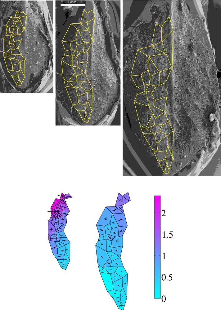
Epoxy resin casts observed by Scanning Electron Microscopy (day 1, day 3, day 5). Red dots (characteristic marker points) were used to divide the leaf blade into polygons and obtain the meshwork (1st row). The meshwork with an extreme direction of deformation calculated for an exemplary Arabidopsis leaf in 48-h time intervalsis represented with crosses. The color map represents the areal growth rate (second row) (color online).
2 Material and methods
2.1 Plant material and growth conditions
Arabidopsis thaliana ecotype Columbia-0 (Col-0) plants were grown in pots in short days (9 h day; 15 h night), at temperature between 19–21 oC, illumination 60 μmol m–2 s–1. In such growth conditions, aerial rosettes are formed in the axils of the oldest cauline leaf of plants 16–20 weeks after germination [1]. The third or fourth leaves of such aerial rosettes were used in the investigation. All the leaves were in the expansion phase of development [15].
We examined the adaxial epidermis of leaf blade at three time points at 48-h time intervals (referred to as days 1, 3, 5) for three leaf blades. The examination was performed with the aid of a non-invasive sequential replica method [16]. Briefly, the replica was taken from the leaf surface using silicon dental polymer. The replicas were next used as forms for epoxy resin casts, which were observed in Scanning Electron Microscopy (SEM). An effort was made to obtain the top view image from each cast. This method gives very good results only for three time points. If more time steps are applied, the leaf blade growth slows down. The experimental data were sufficient to propose a model of growth for the leaf blade.
2.2 Data analysis
In order to compute growth variables from the consecutive images of an individual leaf (day 1–5), we specified a mesh consisting of polygons. The polygons were defined by three to nine points that can be recognized at consecutive images of a growing leaf (see red dots in Fig. 1). These points were either vertices (three-way junctions of anticlinal epidermal cell walls) or geometric centers of trichome bases. Each polygon consisted of several cells. These empirical data were used to compute growth variables. Based on the polygon deformation during leaf growth, we calculated the directions of maximal and minimal deformation for individual polygons using the Goodall and Green formula [17], which are further called extreme directions of deformation (EDDs). The Goodall and Green method is dedicated to triangles. However, we applied it for polygons because, although the triangulation of the leaf blades would be possible, many of triangles would be far away from equilateral ones. This would imply more errors than the adapted approximation in the Goodall–Green method for the polygons. For the modeling, we assumed that the EDDs represent PDGs. We also calculated the relative area increment (Ia) for each polygon according to the formula , where St is the surface of a chosen polygon in t time point.
2.3 Modeling
First, we determined the curvilinear coordinate system in which the leaf is growing. Two coordinate systems with one axis of symmetry have been applied to plant organs [18,19], i.e. paraboloidal and logcosh curvilinear orthogonal coordinate system. We chose the paraboloidal one, which is simpler, and then we adjusted the location of the leaf blade assuming velocity functions for all its points. The postulated velocity functions were non-stationary where their components were sigmoid functions. In statistical analysis, we employed the t-test to check how well the chosen coordinate system fits to empirical data (comparing empirically obtained EDDs with versors of the coordinate system – PDGs). Having velocity functions in a curvilinear coordinate system, we applied the growth tensor to develop the growth model for the Arabidopsis leaf. For calculations and visualization of virtual leaf blade growth, original codes were written in MATLAB (MathWorks). All the statistical analyses were performed with the aid of STATISTICA 10 (StatSoft).
3 Results
3.1 Empirical data on leaf blade growth
First we computed the relative area increment (Ia) and EDDs which are represented in Fig. 1 as colormaps and the crosses for the exemplary mesh of polygons at the surface of growing leaf. These empirical data show that:
- • there is a gradient of Ia along the midrib (the lowest rates are in the distal leaf portion);
- • growth is more anisotropic in the distal leaf portion than in proximal;
- • the area increment is lower during the second time interval.
3.2 Natural coordinate system and GT field for Arabidopsis leaf
Based on the computed EDDs, we assumed that the appropriate coordinate system for the arabidopsis leaf is paraboloidal. The explicit form of the paraboloidal coordinate system is:
| (1) |
| (2) |
| (3) |
We further call this system the leaf natural coordinate system (L-NCS [u,v]).
Next, we searched for the correct location of the growing leaf blade in the L-NCS(u,v) (Fig. 2).

Leaf natural coordinate system applied to a growing leaf. A) day 1, B) day 3 (color online).
Both stationary GT field and non-stationary GT field were considered (Fig. 3). First, we showed, with the ANOVA test (Table 1), that there were no significant differences between the analyzed leaves in both considered time intervals (comparing angles between EDDmax and versor in the u direction, eu).
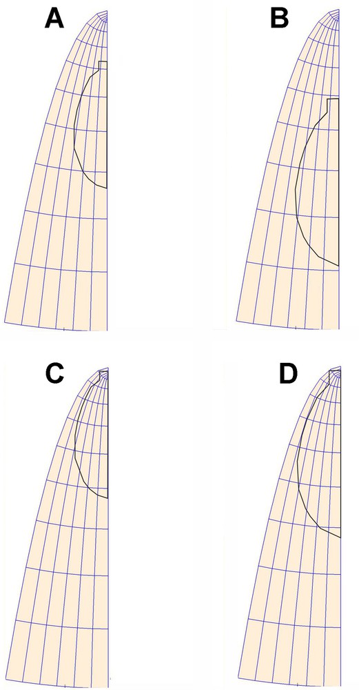
Schematic representation of the leaf in the initial stage of the simulation (A), in a non-stationary GT field (C), in a stationary GT field. (B, D) Final stage of simulation, non-stationary and stationary GT fields, respectively (color online).
Comparison of the considered Arabidopsis leaves in each time interval: (A, C) from day 1 to day 3; (B, D) from day 3 to day 5. (A, B) are computed for a non-stationary GT field, (C, D) for a stationary GT field (the one-way ANOVA analysis for angles between EDDmax and eu in the considered three leaves). The differences between the analyzed leaves are statistically non-significant (significant level 0.05).
| ANOVA test | ||
| F-value | P | |
| A | 0.005 | 0.995 |
| B | 2.854 | 0.063 |
| C | 0.563 | 0.572 |
| D | 2.208 | 0.116 |
If the natural coordinate system were chosen correctly, the EDDs calculated for all the polygons would agree with the versors (eu, ev) of the system. Therefore, angles were measured between the maximal direction of deformation (EDDmax) and eu at geometric centers of all polygons. This was done for both time intervals for the examined leaves in both stationary and non-stationary GT fields. In order to determine whether there were significant differences between orientations of EDDmax and eu (see mean and median values in Table 2), the t-test for dependent samples was performed (significance level: 0.05). The paired t-test showed significant differences between EDDmax and eu in a stationary GT field (Table 2 C, D), and no significant differences in a non-stationary GT field (Table 2 A and B). Statistical analysis shows that the assumed non-stationary GT field operating in the chosen L-NCS (u,v) is the correct one and describes well the growth of the leaf blade. We have proven that there are no statistically significant differences between the EDDs calculated directly from the empirical data and those assigned by coordinate system (eu, ev) during the virtual leaf blade growth.
Paired t-test for each individual polygon for the differences between EDDmax and eu for the growing leaf blades of A. thaliana Col-0 (experimental and model data). Calculation performed for two time intervals of leaf growth: (A, C) from day 1 to day 3; (B, D) from day 3 to day 5. A, B are computed for a non-stationary GT field, C, D for a stationary GT field. Notation: SE–standard error, n–sample size. Each class of angles was considered separately.
| Paired t test | ||||
| Mean ± SE | n | t-value | P | |
| A | 3.43 ± 2.38 | 90 | 1.50 | 0.14 |
| B | 6.84 ± 2.98 | 85 | 0.59 | 0.56 |
| C | 1.76 ± 2.46 | 90 | 2.78 | 0.01 |
| D | 7.99 ± 3.23 | 85 | 2.47 | 0.02 |
In the non-stationary GT field, the pattern of PDG trajectories computed from the model changes during leaf blade growth, because the GT field moves with respect to the leaf (the focus of the coordinate system moves away from the leaf).
Having the L-NCS, we assumed displacement velocity functions V for all the points of a growing leaf. In 2D, the velocity functions (both are sigmoid, see also [20]; Fig. 4A) in two orthogonal directions (u,v) are:
| (4) |
| (5) |
| (6) |
| (7) |
| (8) |
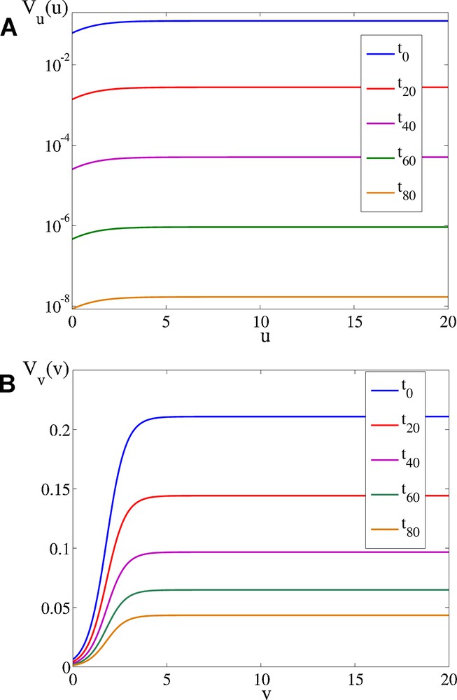
Velocity functions. A) in the u direction (semi logarithmic scale), B) in the v direction (color online).
The velocity functions are presented in Fig. 4 for several time steps. The velocity function in the u direction is presented on a semi logarithmic scale, because its value decreases rapidly in time. The general expression for the velocity function for the Arabidopsis leaf in the i direction is:
| (9) |
The graphical representation of R1 in 2D, calculated from the above equations of the velocity functions, is presented in Fig. 5. The spatial variability from isotropic to anisotropic growth is apparent. The considered leaf blade moves through this field, and accordingly R1 in the u direction changes its value, while R1 changes in the u direction are much smaller.

Anisotropy of the growth tensor field represented by indicator (color online).
3.3 Application of the non-stationary GT field in the simulation model of Arabidopsis leaf growth
Further, using the GT, we created also a model of growing Arabidopsis leaf in the expansion phase of its development. The results of such modeling are presented in Fig. 6. We assumed that an initial shape of a virtual leaf blade is a simplified outline of real leaf blade (neglecting the leaf margin serration). Such virtual blade was placed in the defined non-stationary GT field, and five exemplary time steps of its growth are presented. The simulation shows a cessation wave of Ra that moves from the proximal to the distal part of the leaf (see also Movie 1). In the first time interval, the value of Ra, computed between the first and the second time step of the simulation, is generally higher than in the following intervals, and attains its maximal value in the proximal part of the leaf blade. The gradient of Ra is the steepest in the first time interval and, in the following intervals, it gradually decreases. Similar growth changes take place in the real leaf blade (compare Fig. 1, 2nd row, and Fig. 6). Therefore, we conclude that our model functions properly.
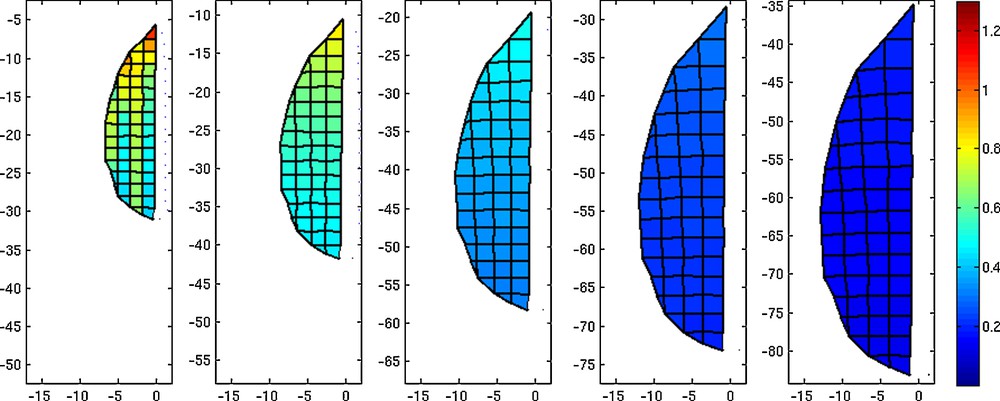
Five time stages of the growth of a virtual leaf. The current position of the growth tensor field is represented by the axis. The color map of polygons represents the areal growth rate Ra (color bar in arbitrary units).
The proposed model can also be used to predict the growth rate along the main leaf axis, i.e. along the midrib. Movie 2 shows the changes in Rl computed in the direction parallel to the leaf midrib. It shows that the maximum Rl is in the most proximal part of the leaf blade. In the following steps, this value decreases and the Rl distribution along the midrib becomes uniform. We can also predict Rl in other directions, for example the Rl in the direction perpendicular to the midrib (u direction in L-NCS) (Movie 3). In this case, no maximum appears. Rl in u direction is uniform and decreases with time.
4 Discussion
Here, we present the modelling method adopted to leaf blade expansion that can be used also to model the growth of other, symplastically growing plant organs. To specify the model variables, we need the experimental data on displacement velocities of marker points on the organ surface. Having the empirically obtained displacement velocities, we can formulate appropriate velocity functions in the natural coordinate system (NCS). The system is natural if the orientation of EDDs obtained using the Goodall–Green formula are in agreement with the orientation of versors in NCS. The velocity functions are therefore combined with the NCS and the estimations between both are mutually dependent. The calculations are much easier in a stationary field case because the versors are independent of velocity functions; nevertheless, non-stationary fields can be also modeled.
There exist several models of leaf blade growth. Computer analysis of leaf growth was first performed by Erickson [8]. This analysis was based on empirical data acquired from a Xanthium pensylvaticum leaf and the method of analysis proposed by Richards and Kavanagh [21]. A set of points (landmarks) was placed on the surface of the growing organ. These points changed position due to surface expansion. The displacement velocity vectors of points were used to estimate growth gradients within the plant organ. A discrete approach was also used for modeling leaf growth [22]. Wang et al. [23] created a model for the Xanthium leaf, similar to ours, but they consider only the growth simulation without maps of the growth rate changes. Their animation corresponds to three days of leaf growth. Kennaway et al. [24] studied the role of tissue polarity and differential growth in the generation of the shape. Their model includes interactions between regulatory factors (hormones), velocity field (generating displacement field used to calculate the field of volumetric growth) and elasticity (used to compute the resultant deformation of the cells). Dupuy et al. [25] modeled the cell–cell interactions with the genetic background. They focussed on the distribution of trichomes on the leaf surface, while, in our approach, we focus on the growth rate maps and the change of the general shape of the whole leaf blade. Backhaus et al. [26] and Bilsborough et al. [27] in turn model only the margin of the Arabidopsis leaf accounting for the serration, and the geometric form of the leaf, and combine it with single-metric shape parameters for different mutants [26] or the auxin distribution and gene expression [27]. Since our model neglects the leaf margin serration, combining their modeling with ours, one can obtain a wider description of the Arabidopsis leaf growth and form.
In the present paper, first the velocity field V for the displacement of points and the appropriate coordinate system was defined. This allowed us to calculate the growth tensor field in which the leaf blade is placed. This field is non-stationary and the numerical calculations are unavoidable. The field is dedicated to experimental data coming from Arabidopsis leaves. We obtained the quantitative data of the velocity field with the aid of the sequential replica method [16]. The model can be briefly described as follows. The leaf grows in a non-stationary GT field according to the velocity functions given by Eqs (4, 5). The field moves with respect to the leaf along the leaf midrib (Fig. 6). The velocities decrease in time with factors a, b (Eqs. (6, 7)).
We postulate the velocity functions that describe the displacement velocities of the points defined on the leaf blade. These velocity functions influence the actual position of the leaf blade in the coordinate system. We have proven that there are no statistically significant differences between the orientation of EDDs calculated directly from the empirical data and those assigned via coordinate system (eu, ev) during the virtual leaf blade's growth. We showed that the empirically obtained orientation of EDDs fit the principal direction of growth in both examined time intervals. The velocity functions are valid only in the curvilinear coordinate system, in this case paraboloidal, and therefore we regard this system as the natural coordinate system for Arabidopsis leaf blade (L-NCS). The presented model of the leaf blade growth can be used to predict the growth in any intermediate time step and in any direction during the expansion stage of leaf development. The velocity functions are sigmoids and they can be modulated via the parameters defined in Eq. (9), to achieve the empirically obtained values.
Up to now, in the description of plant growth with the aid of GT, only the stationary GT field was considered, in which the growth tensor was steady in time and space. Such a stationary GT field was applied to the modeling of growth of root and shoot apices [9–11]. In the present model that assumes a non-stationary GT field, the leaf moves through the field (spatial changes) and growth is decreasing in time (temporal changes). This property of growth can be obtained by using the specific velocity functions. We considered also the stationary GT field, by placing the growing leaf in the focus of the coordinate system, but we falsified this kind of approach: there are significant differences between orientation of versors in L-NCS and the empirically obtained EDDs.
The stationary GT field was applied to the organs self-maintaining their shapes: root and shoots. Leaf is beyond this description, the leaf blade changes its shape in time and space and the non-stationary GT field can explain this feature. To conclude, one can say that the fact that plant organs self-maintain their shapes can be described by a stationary GT field, and plant organs changing their shapes by a non-stationary GT field.
Our model is in agreement with the results presented by Kuchen et al. (fig. 1 J in [30]) and Remmler and Rolland-Lagan [28] and Walter et al. [29]. The maximum growth rate can be found in the proximal region of the leaf blade, and a gradient of growth rate is observed. Also, the linear growth rates in Movie 2 are similar to those shown in Fig. 1e–i of Kuchen et al. [30]. GT modeling provides also information about growth anisotropy (temporal and spatial dependencies).
The presented model includes a complete kinematic information on the leaf blade growth. We are able to calculate growth rates in any direction as well as growth anisotropy. We can also simulate changes in leaf blade shape and size during its growth. The starting point of the modeling is the determination of the displacement velocity functions, which in the case of the Arabidopsis leaf blade are sigmoids (Fig. 4A in [20]). The next important issue is to adjust the appropriate coordinate system, defining the principal directions of growth. These two ‘variables’ (velocity functions and natural coordinate system) provide a full kinematic description of growth, but the numerical calculations are unavoidable.
Disclosure of interest
The authors declare that they have no conflicts of interest concerning this article.
Acknowledgements
The authors specially thank Prof. Dorota Kwiatkowska and Dr Agata Burian (University of Silesia) for discussion and critical reading of this text.
Dr Ewa Teper from the Laboratory of Scanning Electron Microscopy, Faculty of Earth Sciences, University of Silesia, is acknowledged for her help in the preparation of SEM micrographs.Author contributions: M.L. designed and performed research, analyzed data, prepared model and wrote the paper, A.P-S. performed statistical analysis and analyzed data, J.E. and J.P. experiments.Funding: The research was partially funded by a grant from the National Science Centre [grant number N N303 8100 40] in 2011–2012 (ML, JE), and by the Polish Ministry of Science and Higher Education [grant number N N303 3917 33] in 2007–2010 (JP). The funders had no role in study design, data collection and analysis, decision to publish, or preparation of the manuscript.