

1 Introduction
The different ways to represent a biological signal are aiming both to:
- • explain the mechanisms having produced the signal;
- • facilitate its use in medical applications or in life sciences.
The biological signals can come from electrophysiologic signal sensors like ECG, arterial pulse sensors, etc., or from molecular devices like mass or NMR spectrometry, etc., and have to be modelled and compressed for an efficient medical use by clinicians and to retain only the pertinent information about the mechanisms at the origin of the recorded signal for the researchers in life sciences, or restored to be interpreted, e.g., in telemedicine. If the recorded signal is periodic in time and/or space, the classical compression processes like Fourier and wavelet transforms give good results concerning the compression rate, but bring in general no supplementary information about the interactions between elements of the living system producing the studied signal. Here, we define a new transform called Dynalet based on Liénard differential equations, which are susceptible to model the mechanism that is the source of the signal and we propose to apply this new technique to real signals like ECG, arterial pulse and mass or NMR spectrometry. We will recall in Section 2 the classical Fourier and wavelet Haley transforms from the point of view of differential equations, and then, we present in Section 3 the prototype of the Liénard equations, i.e. the van der Pol equation. In Section 4, we will define the Dynalet transform, and then describe in Sections 5 to 8 the biological applications.
2 Fourier and Haley wavelet transforms
The Fourier transform comes from the desire of Joseph Fourier [1], in 1807, to represent in a simple way functions used in physics, notably in the frame of heat propagation modelling. He used a base of functions made of the solutions to the simple not-damped pendulum differential equation (cf. the trajectory on Fig. 1):
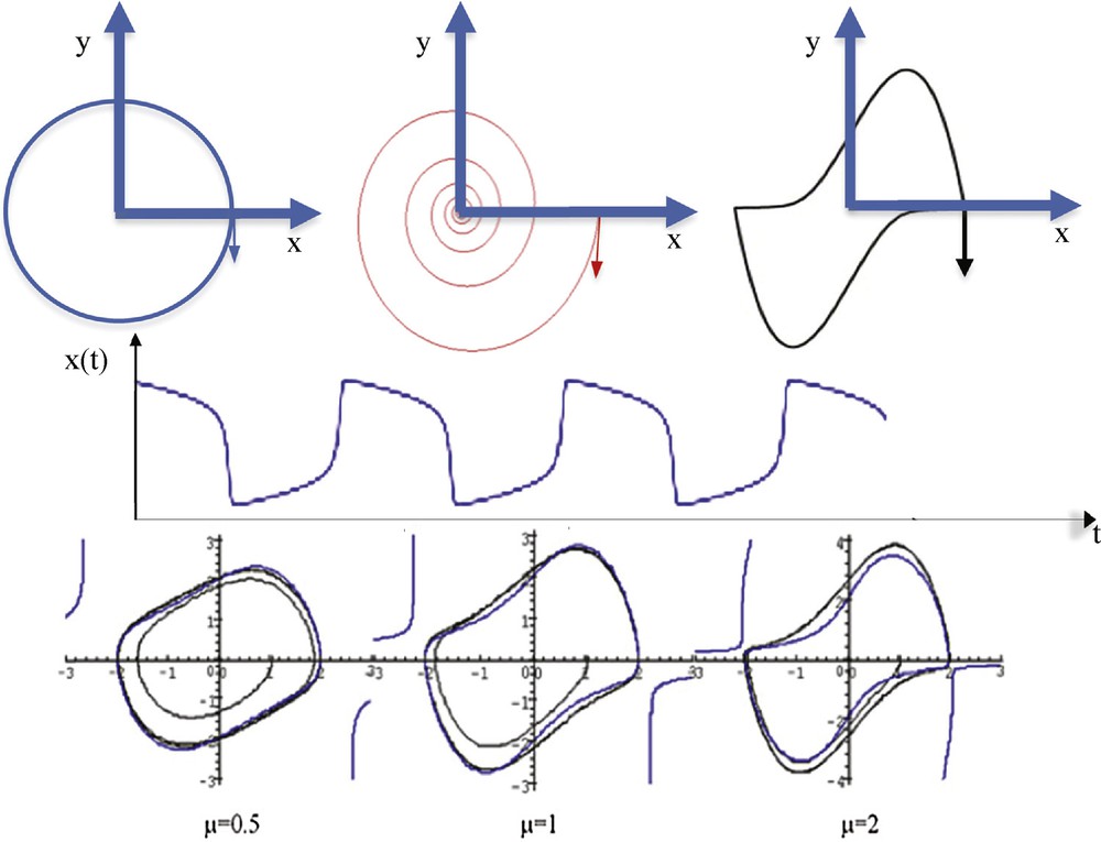
(Color online.) Top left: a simple pendulum trajectory. Top middle: a damped pendulum trajectory. Top right: van der Pol limit-cycle (μ = 10, ω = b = 1). Middle: relaxation oscillation of the van der Pol oscillator with μ = 5, ω = b = 1. Bottom: representation of the harmonic contour lines HvdP(x,y) = 2.024 for different values of μ.
By using the polar coordinates θ and ρ defined from the variables x and z = −y/ω, we get the new differential system:
After the seminal theoretical works by Meyer [2,4], Daubechies [3] and Mallat [5], Haley [6] used in 1997 a simple wavelet transform for representing signals in astrophysics. He used a base of functions made of the solutions to the damped pendulum differential equation (cf. the trajectory on Fig. 1):
By using the polar coordinates θ and ρ defined from the variables x and z = −y/ω – τx/ω, we get the differential system:
The polar system is dissipative (or gradient), its potential function being defined by P(θ,ρ) = −ωθ + τρ2/2. The general solution x(t) = k e−τtcosωt, z(t) = k e−τtsinωt has three degrees of freedom, k, ω and τ, the last parameter being the exponential time constant responsible for the pendulum's damping.
3 The van der Pol system
For the Dynalet transform, we propose to use a base of functions made of the solutions to the relaxation pendulum's differential equation (cf. the trajectory on Fig. 1, top right), which is a particular example of the most general Liénard differential equation:
- • μ appears as an anharmonic term: when μ = 0, the equation is that of the simple pendulum, i.e., a sine wave oscillator, whose amplitude depends on the initial conditions. Relaxation oscillations are observed even with small initial conditions (Figs. 1 and 2), with a period T equal to 2π/Imβ near the bifurcation value μ = 0, where β is eigenvalue of the Jacobian matrix J of the van der Pol equation at the origin:
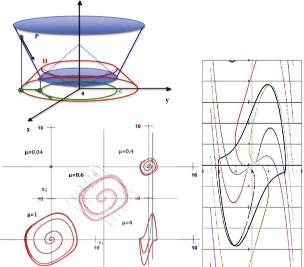
(Color online.) Top left: representation of the potential P and Hamiltonian H on the phase plane axis (xOy). Bottom left: limit-cycle of the van der Pol equation for different values of μ (from [16]). Right: isochronal landscape surrounding the van der Pol limit-cycle (μ = 2, ω = b = 1; period T ≈ 7.642).
The characteristic polynomial of J is equal to: β2–μβ + ω2 = 0, hence β = (μ ± (μ2–4ω2)1/2)/2 and T ≈ 2π/ω + πμ4/2ω3:
- • b looks as a term of control: when x > b and y > 0, the derivative of y is negative, acting as a moderator on the velocity. The maximum of the oscillations amplitude is about 2b, whatever the initial conditions and values of the other parameters are. More precisely, the amplitude ax(μ) of x is estimated by 2b < ax(μ) < 2.024b, for every μ > 0, and when μ is small, ax(μ) is estimated by: ax(μ) ≈ (2 + μ2/6)b/(1 + 7 μ2/96) [12,13]. The amplitude ay(μ) is obtained for dy/dt = 0, i.e. is approximately for x = b, then ay(μ) is the dominant root of the following algebraic equation: HvdP(b,ay(μ)) = 2.024;
- • ω is a frequency parameter: when ω >> μ/2 >> 1, the period T of the limit-cycle is determined mainly by the time during which the system stays around the cubic function where both x and y are O(1/μ), T being roughly estimated to be T ≈ 2π/ω, and the system can be rewritten as: dχ/dt = ζ, dζ/dt = −ω2χ + μ(1–χ2/μ2)ζ ≈ −ω2χ + μζ, with the change of variables: χ = μx/b, ζ = μy/b.
4 The Dynalet transform
The Dynalet transform consists in identifying a Liénard system based on the interactions mechanisms between its variables (well expressed by its Jacobian matrix) analogous to those of the experimentally studied system, whose limit-cycle is the nearest (in the sense of the Δ set or of the mean quadratic distances between sets of van der Pol points and experimental points having the same phase, sampled respectively from the original signal and the van der Pol limit-cycle) to the signal in the phase plane (xOy), where y = dx/dt. We can notice that the Jacobian interaction graph of the van der Pol system contains a couple of positive and negative tangent circuits (called regulon [10]). Practically, for performing the Dynalet transform, it is necessary to choose:
- • the parameters ω and μ such as the period of the van der Pol limit-cycle equals the mean period of the original signal;
- • a translation of the origin of axes, in order to fix the first van der Pol point on its limit-cycle identified, by convention, at the first signal point (corresponding to the mean baseline value of the original signal);
- • a homothety on these axes defining their scales, by minimizing the distance between two sets of points from both van der Pol and original signals.
By repeating this process for the difference between the original signal and the van der Pol limit-cycle, it is possible to get successively a polynomial approximation of the fundamental reconstructed signal and of its harmonics.
The potential and Hamiltonian parts PvdP and HvdP used for this transform can be calculated following [7–9]. For example, for μ = 1 (respectively [resp.] μ = 2), the corresponding polynomials are respectively P1 and H1 (P2 and H2), defined by:
Using this potential–Hamiltonian decomposition, it is possible to calculate an approximate solution S(ki,μi)(t) of the van der Pol differential system corresponding to the ith harmonics of the Dynalet transform, as a polynomial of order 2 + i verifying:
We will search for example for the approximate solution x(t) = S(1,1)(t) as a polynomial of order 3 in the case μ = 1:
The polynomial coefficients ci's above represent both the potential and Hamiltonian parts of the van der Pol system and they can be obtained by identification with P1 and H1 derivatives [7–11]: dx/dt = −∂P1/∂x + ∂H1/∂y, dy/dt = −∂P1/∂y–∂H1/∂x. Then, we get:
A first example of application of the Dynalet technique can be represented by the mitosis rhythm in lateral cells of the caudal fin in zebrafish [16]: by using the relaxation waves of a van der Pol oscillator (Fig. 3), we can fit better the mitosis curve (represented by the intracellular BrDU concentration evolution on Fig. 4) than when using a sine function.
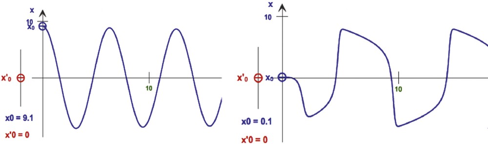
Representation of different waves from van der Pol oscillator simulations (from [15]), from the symmetric type (left, for μ = 0.4, ω = 1, b = 4) to the relaxation type (right, for μ = 4, ω = 1, b = 4).
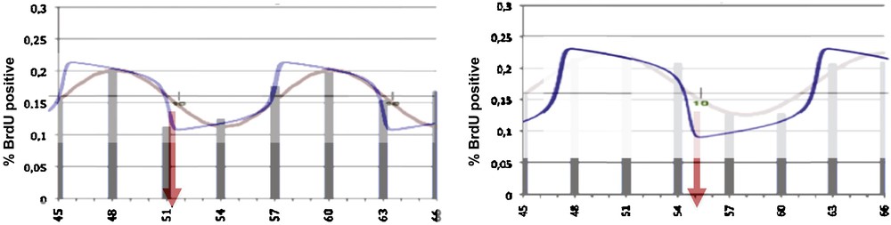
Left: BrdU concentration evolution representing the mitosis rhythm in lateral cells of caudal fin in zebrafish [16], with indication of the nadir (time of the minimum) of the cycle (red arrow), showing a rather good fit with the sine function (red) and a better fit with the van der Pol relaxation wave (blue). Right: same curve for the axial cells, showing a phase shift of the nadir, due to the spatial bell shaped form of the caudal fin. Masquer
Left: BrdU concentration evolution representing the mitosis rhythm in lateral cells of caudal fin in zebrafish [16], with indication of the nadir (time of the minimum) of the cycle (red arrow), showing a rather good fit with the ... Lire la suite
5 Cardiovascular applications
We propose to apply this new technique to real signals like ECG and pulse rhythm. In these both cases, the rhythmic cardiovascular activity results from the summation of cellular oscillators (Fig. 5) located in the cardiac sinus node, which are subject to the control of the bulbar cardiovascular moderator and cardio-accelerator centres, which modulate the sinus signal, integrating the influence of the inspiratory bulbar centre, which causes the appearance of harmonics in the cellular rhythm.
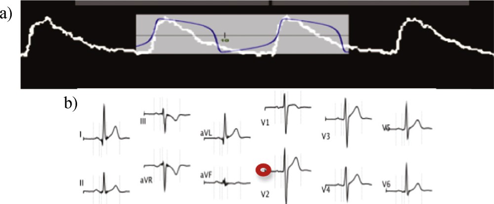
(Color online.) a: van der Pol signal [15] fitting (in blue) the single cardiac cell activity [17] (in white); b: ECG signals recorded for different electrophysiologic derivations (from [18]), with indication (in red) of the baseline.
The Dynalet transform consists in identifying a Liénard system that expresses interactions between its variables through its Jacobian matrix analogous to those of the experimentally studied system, whose limit-cycle is the nearest (in the sense of the distance Δ between sets, or of the mean quadratic distance between points of same phase) to the signal pattern in the phase plane (xOy), where y = dx/dt.
Practically, if the Liénard system is a van der Pol system, it is necessary to execute the following transforms for getting Dynalet approximation from original signal:
- • to estimate the parameters ω and μ such as the period of the van der Pol signal is equal to the mean empirical period (calculated for the original signal);
- • do a translation of the origin of axes in the phase plane;
- • do a homothetic change of the coordinates, in order to match the van der Pol signal to the original signal.
Then the whole approximation procedure done for the ECG signal (Fig. 6a) involves the following steps:
- • suppress the time intervals when the signal was under the critical plateau value Λ of the Levy time λ(ɛ) equal to the time interval during which the signal has passed between 0 and ɛ. This step allows obtaining the QRS complex of the experimental ECG (Fig. 6b and c);
- • fix the value of the parameter μ such as the period of the van der Pol signal is equal to the QRS complex duration;
- • perform a translation of the origin of the (xOy) phase plane and a scaling on the coordinates of the van der Pol signal, so as to adjust them to the maximum of the x QRS complex;
- • finish the approximation with a parameter optimization (parameters ω and b), by matching the QRS complex points to the van der Pol limit-cycle in order to minimize the distance Δ between the interiors of the QRS points set and the van der Pol limit-cycle (denoted respectively by ECG and VDP, with interiors ECG0 and VDP0) in the phase plane:
by using a Monte-Carlo method for estimating the area of the interiors of the linear approximation of empirical points of the Experimental QRS complex and of the van der Pol limit-cycle, calculated from a sample of points in the phase plane, respectively {Ei}i = 1,100 and {Pi}i = 1,100. It is also possible to minimize the mean quadratic distance between the points of the van der Pol limit-cycle and the empirical points having the same phase;
- • repeat the procedure for obtaining the successive harmonics in order to respect, for example, a fixed threshold of 20 dB for the signal-to-noise ratio (SNR) and 10% for the quadratic relative error (QRE);
- • calculate a polynomial approximation of the signal from the quadratic estimate of the van der Pol limit-cycle corresponding to the previous step, e.g., if ω = b = 1:
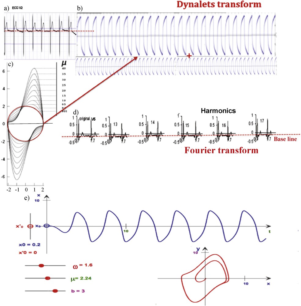
(Color online.) a: ECG signal (V2 derivation); b: decomposition into two temporal profiles respectively of period T and T/2, whose corresponding functions are orthogonal for the integral on [0,T[of the vector product; c: representation of different van der Pol limit-cycles, for different values of μ (from μ = 0.01 in red, to μ = 4, with ω = b = 1); d: Fourier decomposition of the ECG signal (V5 derivation), showing the reconstruction process until the 17th harmonics; e: representation of a relaxation wave from van der Pol oscillator simulations [15], for μ = 2.24, ω = 1.6, b = 3. Masquer
(Color online.) a: ECG signal (V2 derivation); b: decomposition into two temporal profiles respectively of period T and T/2, whose corresponding functions are orthogonal for the integral on [0,T[of the vector product; c: representation of different ... Lire la suite
6 Application to ECG
Let now compare the performance of the Dynalet reconstruction of the ECG V1 signal (given on Fig. 8c) with a Fourier transform having the same number of parameters, that is 5, i.e., the origin abscissa translation, two values of μ (period) and two abscissa scaling ratios for the fundamental and first harmonic of the Dynalet transform; the period, the origin abscissa translation and three values of sine coefficients for the Fourier transform F(x) (Fig. 7), whose equation is:
(Color online.) a: First coefficients of the Fourier transform of the QRS complex: the fundamental and two first harmonics are labelled; b: original QRS complex of the ECG (green) and Fourier (blue) reconstruction with two harmonics matching; c: experimental ECG V1; d: evolution of the Lévy time λ(ɛ) corresponding to the time interval during which the signal passed between 0 and ɛ.
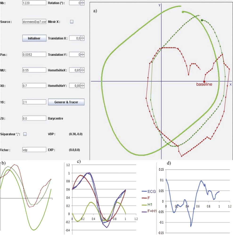
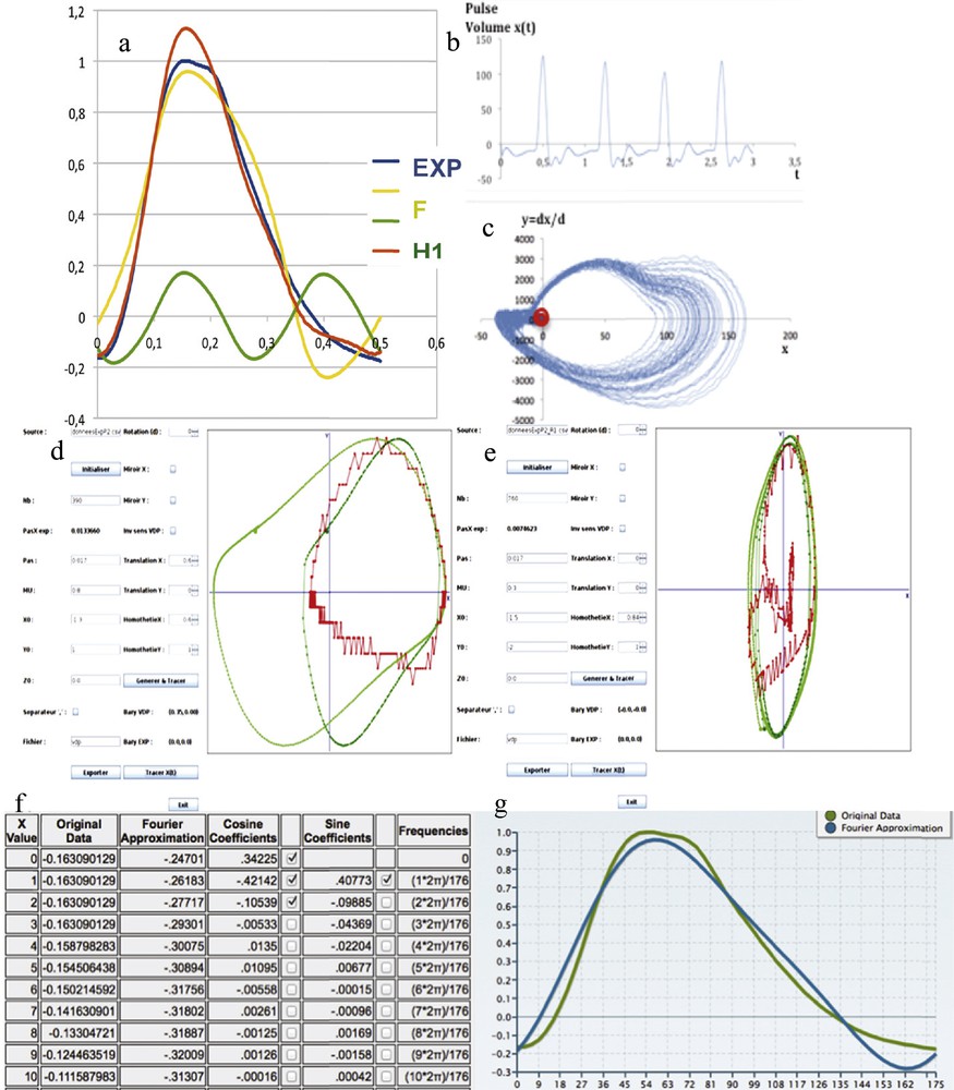
(Color online.) a: Initial position in the phase plane xOy of the van der Pol limit-cycle (in green clear) and ECG signal (in red) and final fit between van der Pol (in dark green) and ECG signal after transformation on the X and Y axes (translation and scaling); first row: b: fundamental component extraction from the original experimental ECG signal (in red), (i) by identifying the phase 0 value on the original V1 derivation in the phase plane xOy, where y = dx/dt, then a sample of 100 points extracted from the mean signal, on the van der Pol limit-cycle having the same period as the pitch of the mean ECG signal; c: match for getting the fundamental Dynalet component (F in blue) and first harmonic (H1 in green), with a transformation in the (xOy) phase plane consisting in translating/scaling x and y axes (as indicated in the left table of a), in order to obtain the best fit for the cost function based on the Δ distance between sampled empirical mean points (blue curve) and the set of points of same phase extracted from the van der Pol limit-cycle; d: subtracting the fundamental plus the first harmonic component (F + H1 in violet) from the sampled original ECG signal (in blue). Masquer
(Color online.) a: Initial position in the phase plane xOy of the van der Pol limit-cycle (in green clear) and ECG signal (in red) and final fit between van der Pol (in dark green) and ECG signal after ... Lire la suite
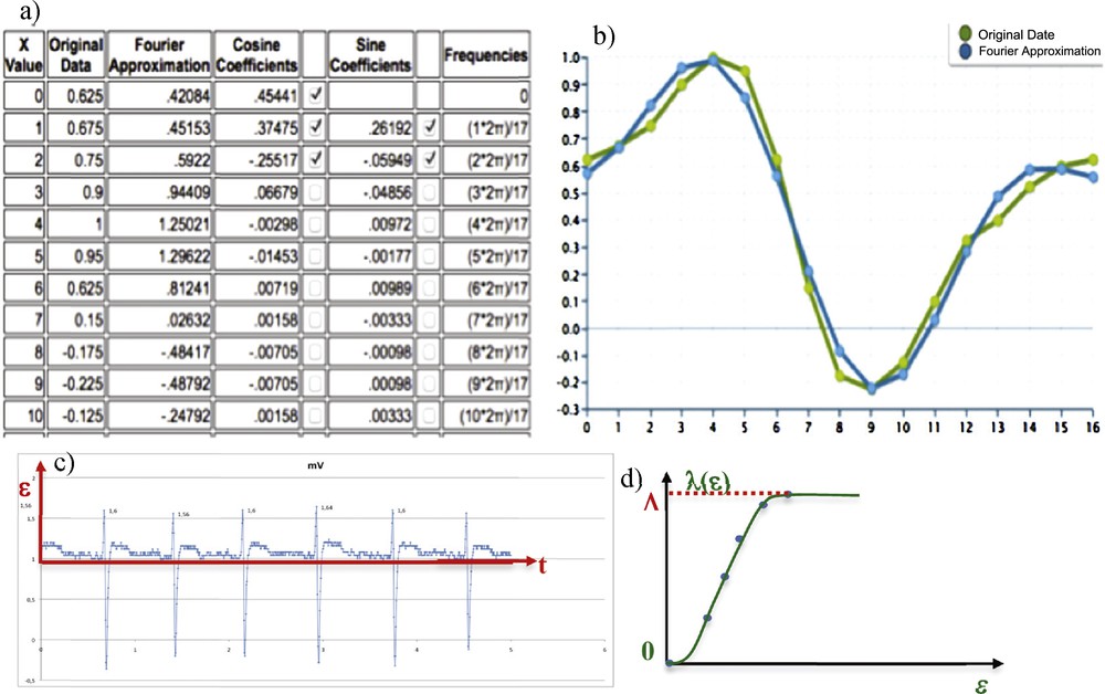
For defining a quantitative assessment of the error between the abscissae of the K original signal observations Xi's (obtained after extraction of the baseline) and their Fourier or Dynalet approximations ξi's, we use the notions of mean square error (MSEX) and signal-to-noise ratio (SNRX) where:
The calculation made for the QRS signal of Figs. 7 and 8 shows, for example, a good Dynalet fit for ordinates values:
In the reconstitution of Figs. 7 and 8, MSEX Fourier = 0.08, SNRX Fourier = 22 dB and MSEX Dynalet = 0.09, SNRX Dynalet = 21 dB. We can notice that this Fourier transform needs six parameters (including the value of the period), while the Dynalet transform requires only five parameters (Fig. 8).
7 The pulse signal
Concerning the pulse signal, the pulse wave is approximated, after identification and extraction of the inter-beats baseline, by using successively the sine functions family (Fourier transform) and the family of the limit-cycles of the van der Pol equation. In the example of the Fig. 11, MSE (resp. SNR) is equal, for the amplitude X, to 0.066 for a Fourier transform having two harmonics with six parameters, and 0.09 for a Dynalet decomposition with one harmonic defined by only five parameters (resp. 24 dB and 21 dB). For the velocity Y = dX/dt, MSE (resp. SNR) is equal to 0.0092 for a Fourier transform with two harmonics and 0.0095 for a Dynalet decomposition with 1 harmonic defined by five parameters (resp. 40.8 dB and 40.4 dB).
(Color online.) a: Dynalet reconstruction of the pulse wave with a fundamental (F) and one harmonic (H1); b: original experimental pulse wave recorded at the level of the dorsalis pedis artery; c: representation of a sequence of pulse waves in the phase plane (amplitude, velocity); d: original pulse (red) and van der Pol (green) signal matching, after an abscissa translation of the origin of the xOy referential and extraction of the points of the base line; e: second matching of the fundamental with a new van der Pol signal of triple period; f: coefficients of the Fourier transform with one harmonics; g: original pulse wave (green) and Fourier reconstruction with one harmonic (blue). Masquer
(Color online.) a: Dynalet reconstruction of the pulse wave with a fundamental (F) and one harmonic (H1); b: original experimental pulse wave recorded at the level of the dorsalis pedis artery; c: representation of a sequence of pulse ... Lire la suite
Given the fact that the Dynalet transform uses asymptotically stable trajectories (limit-cycles) with a differential equation closer to the mechanism of genesis of electrophysiological signals than the simple pendulum used by the Fourier transform, the above-obtained performances for the pulse signal show that the compression rate for Dynalet transform is as efficient as for Fourier transform, while also being more explanatory, than for the Fourier transform.
8 Physiologic applications
One of the reasons explaining the efficacy of the van der Pol equation in representing the cardiac activity lies in the fact that since 50 years and the first models by Noble [19,20], 45 models of the cardiac rhythm have been proposed [21], many of them being based on Hodking–Huxley model, which is closely related to the van der Pol equation (Fig. 9). The van der Pol system is indeed analogous to the 2D-version of the Hodgkin–Huxley equation, called the FitzHugh–Nagumo equation, by just changing the second variable y for the new variable z = y–μx(1–x/√3)(1 + x/√3).
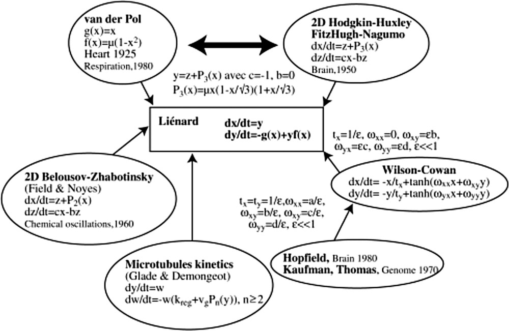
Overview of van der Pol equation in a biological models’ landscape. Interaction graph of these systems contains in general a couple of positive and negative tangent circuits (called “regulons” in [22]).
The explanatory power of the Dynalets in the case of physiologic signals comes also from the fact that cardiac and respiratory rhythms are regulated through interaction loops (called “regulons” in [22]) having one activation, one inhibition and one auto-catalysis, in interaction with the same structure controlling the respiration:
- • the bulbar cardio-moderator CM (resp. cardio-accelerator CAC) inhibits (resp. activates) the sinus node (S);
- • the sinus node activates (resp. inhibits) the CM (resp. CAC) via the peripheral chemoreceptors, and auto-activates itself;
- • the expiratory neurons (E) inhibit the inspiratory ones (I);
- • the inspiratory neurons activate expiratory ones (Fig. 10).
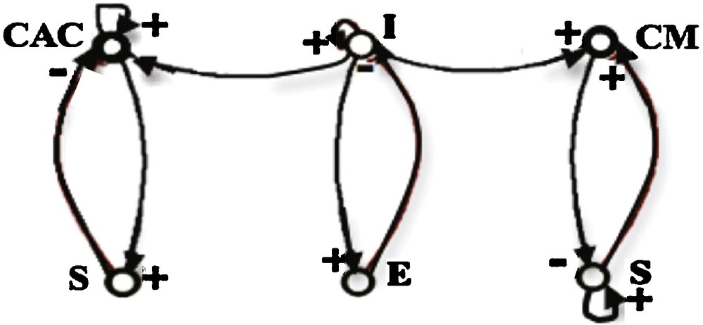
Interaction graph of cardiac (CM, CAC, S) and respiratory (E, I) systems.
Biological rhythms other than the ECG or pulse can be interpreted and compressed using Liénard equations and the Dynalet transform, like the respiratory rhythm or the single cardiac cell activity, which represent good examples of a relaxation wave (Fig. 5a and [23,24]), as well as pulse activity (Fig. 11). In summary, the main advantages of the Dynalet transform on the Fourier transform in the case of periodic physiologic signals are:
- • the limit-cycles of the Liénard systems, like those of the van der Pol system, are asymptotically stable, unlike those of the simple pendulum of Fourier transform, which are asymptotically unstable because the simple pendulum is a conservative Hamiltonian system. In both cases, these trajectories have algebraic approximations;
- • the approximating system in the case of the Dynalet transform explains the mechanism genesis of the signal; for example, in the case of the heart, the van der Pol system has the same interaction structure as the cardiac system;
- • the trajectories of the Dynalets can break the rotation symmetry of the simple pendulum, which makes them more likely to approximate the asymmetrical biological waves, like the relaxation waves.
9 Non-periodic protein spectrum signal
In addition to the compression of periodic signals, another application of the Dynalet transform is the compression of a non-periodic signal. If the mechanism of signal generation is of Liénard type, for example a relaxation in a magnetic field in case of NMR spectroscopy [25] (giving signals of type T1 and T2, which are functions of lifetime of a given energy state, hence of a relaxation rate) or in an electric field in the case of mass spectroscopy [26] (giving signals of relaxation occurring by fragmentation of a molecule, in order to produce ions of lower masses), and even if the signal is a response in the form of isolated peaks, it can approximated by the Dynalet processing. If the peaks are very asymmetric (Figs. 12 and 13), of relaxation type, it is possible to obtain by periodization an approximate polynomial representation of any desired order in the space of the solutions to a Liénard equation. A good example of this type of application is given by the approximation of the spectrum of a protein, observable by NMR spectroscopy or by mass spectrometry.
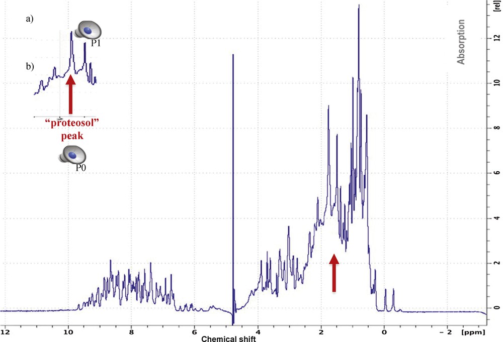
(Color online.) a: Original protein NMR spectroscopy signal; b: extraction of a peak P0 called “proteosol” (because it sounds like a sol) allowing it to be isolated and processed by the Dynalet transform (red arrow). All the peaks (like P1) surrounding the “proteosol” peak P0 are also processed and can be heard.
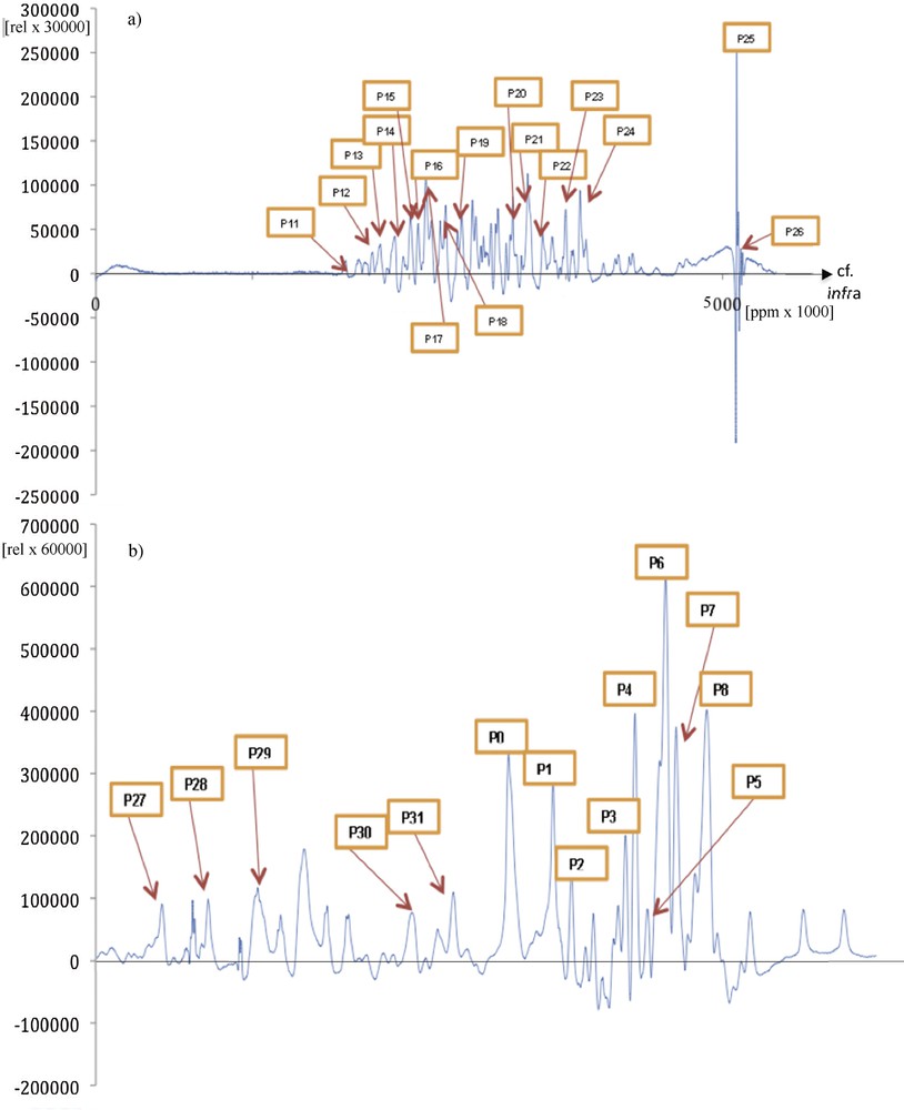
(Color online.) a: Original protein NMR spectroscopy signal; b: extraction of a peak P0 called “proteosol” (because it sounds like a sol) allowing it to be isolated and processed by the Dynalet transform (red arrow). All the peaks (like P1) surrounding the “proteosol” peak P0 are also processed and can be heard.
10 Dynalet transform of a peak from a protein NMR spectroscopy signal
By focusing on the peak indicated by a red arrow red on Fig. 12, we will perform both the Dynalet transform (Fig. 14) and the Fourier transform (Fig. 15). We recall that the level of the mean square error (MSEX) and of the signal-to-noise ratio (SNRX) of these transforms is calculated from the formulas:
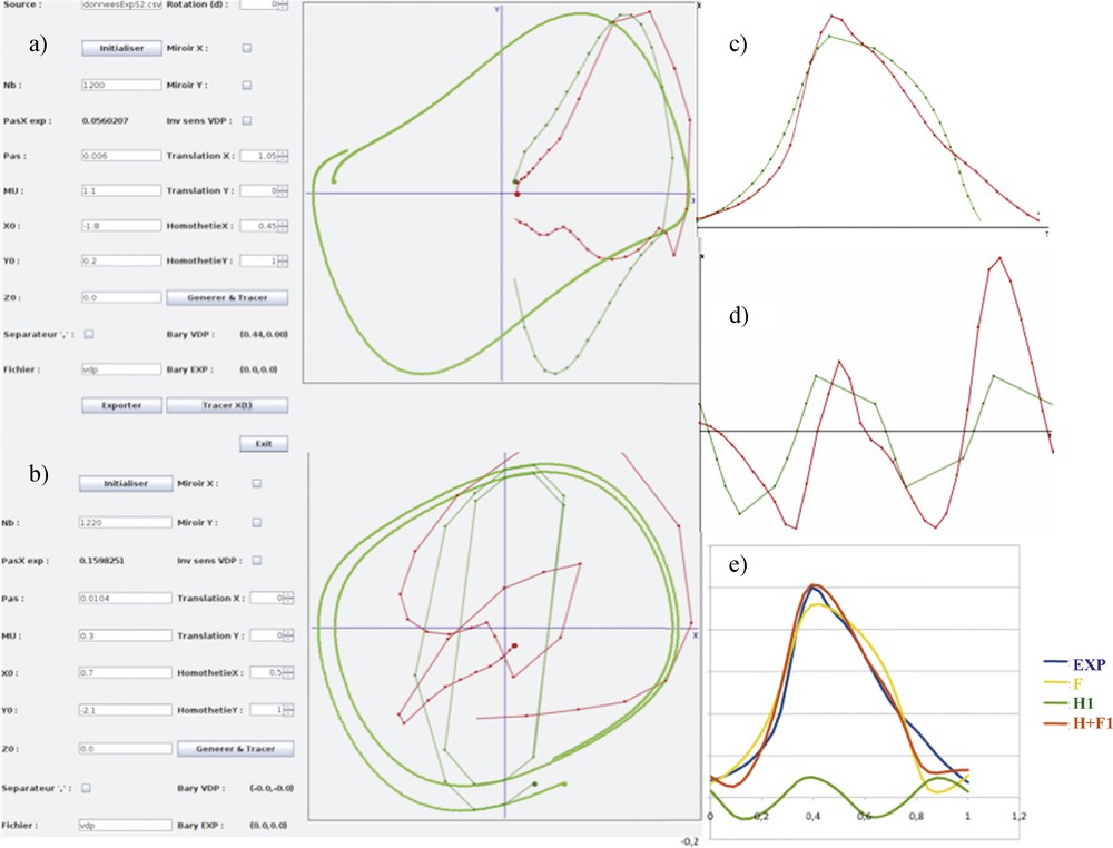
(Color online.) a: Original empirical protein signal of Fig. 12 (in red) matching the van der Pol limit-cycle (in dark green); b: first harmonic signal matching the first harmonic of the van der Pol signal; c: fundamental temporal original signal (in red) matching the van der Pol signal (in green); d: harmonic temporal original signal; e: superposition of the different signals: empirical in blue, fundamental in yellow, first harmonic in green and reconstructed signal in red.
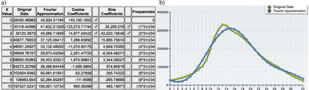
(Color online.) a: Fourier coefficients (fundamental and harmonic); b: reconstruction of the original data (in green) by the one harmonics Fourier transform (in blue).
Following [27], the quality of the reconstitution of the signal can be qualified of low, but it is in general sufficient for performing an efficient surveillance of chronic diseases with protein defects using e-health systems at home (i.e., doing a fusion of actimetric data with metabolic information fixing the gravity level of the disease as the progressive entrance into complications):
- • > 40 dB SNR = excellent signal;
- • 25 dB to 40 dB SNR = very good signal;
- • 15 dB to 25 dB SNR = low signal;
- • 10 dB to 15 dB SNR = very low signal;
- • 5 dB to 10 dB SNR = no signal.
The Fourier transform allows to obtain the reconstruction of a compressed signal XF(t) with one harmonic (Fig. 15), equal to:
One can see on Fig. 15 the quality of the reconstruction of the original data (in green) by the one harmonic Fourier transform (in blue).
11 Toward a protein “stethoscope”
The identification of proteins by their spectrum allows for example the construction of complex genetic control networks, such as those found in the regulation of the immune system [28–31], where key proteins are effectors of the genetic expression (activators or inhibitors) and may be subject to pathologic conditions, leading to up- or down-expressions. These regulatory interactions lead to abnormal protein or protein complexes concentrations in excess or lacking, and spectroscopy peaks indicating these pathologic defects can be treated by the Dynalet approach. Of course, other alternative techniques for estimating protein spectra already exist, like kernel functional estimation tools [32–37], but there are not related to the mechanism of production of the protein signal (Fig. 16).
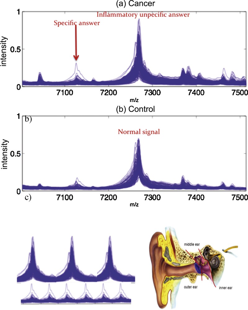
(Color online.) a: Protein spectral data from mass spectrometry showing the response of a patient with cancer [32]; b: that of a normal patient [32]; c: the periodization of the spectrum signals and their transformation into an audible sound.
The Dynalet transform applied to protein data can be considered as a real protein “stethoscope”, which would give sense to numerous metabolic data, which, although very heavy in terms of information (about 5 Go per patient in a modern hospital), are in general not queried and used by clinicians (especially in emergency) and hence remain in the big patient centred data bases, often true cemeteries full of unused data.
In the beginning of the 19th century, René Laennec invented the modern stethoscope and described the thoracic sounds in his Traité de l’auscultation médiate (1819) [38], converting into a synthetic functional information for the ear what physicians were previously describing at numerous anatomic and physiologic levels with their eyes, hence creating the modern medical diagnosis based on the auscultation.
We propose to follow the same methodology, by representing the spectral information from NMR and mass spectroscopy into signals converted into sounds (for example, the signal reconstructed on Fig. 14 sounds like a non-harmonic “sol” of the chromatic scale, for which reason we have called it “proteosol”), expecting that this “protein melody”, whose peaks (see supplementary material to hear the peaks indicated on Fig. 13) are well enhanced by the human ear at the cochlear level, serve to differentiate pathologies from the normality and remain in the memory of the clinicians (e.g., in the context of a rapid medical decision in an emergency service or of a discussion about a complex case in a cancer staff) as quantitatively correlated and semantically associated with precise metabolic diseases, in order to compensate:
- • the complexity of the interactions between proteins and with their substrate and regulation molecules;
- • the overflow of information provided by numerous devices like NMR and mass spectroscopy.
12 Conclusion
Generalizing compression tools like Fourier or wavelets transforms is possible, if we consider that non-symmetrical biological signals are often produced by relaxation mechanisms. In this case, we can propose for the dynamical systems modelling these biological signals Liénard-type differential equations, like the van der Pol equation (or its “sister” equation, the FitzHugh–Nagumo equation, Fig. 9) classically used to model relaxation waves and, more generally, non-symmetrical biological relaxation systems often produced by mechanisms based on interactions of regulon type (i.e., possessing at least one couple of positive and negative tangent circuits inside their Jacobian interaction graph [22]) [23,24].
The corresponding new transform, called the Dynalet transform, has been built in the same spirit as the wavelet transform [2–6,39] (used for example for representing solutions to turbulent systems, like Burger's equation [40,41]), the Hanusse transform [42], or the methodology proposed for estimating Tailored to the Problem Specificity mathematical transforms [43–45]. Some preliminary results [46] have been already published and further applications will be published in future articles. As for the Fourier and wavelet transforms, a fast estimation of the Liénard coefficients (calculable using potential–Hamiltonian decomposition techniques [7–11]) is needed by the fast Dynalet transform and could be possible following the neural networks methodology [47,48]. Then, the Dynalet transform will be for example very useful for compressing in real time the signals coming from e-health systems necessary to the fusion between actimetric and physiologic data recorded at home, with genetic and protein information coming in general from hospital records, in order to perform adequate personalized surveillance and trigger pertinent alarms without false alerts [49–51], hence concretizing in medicine the approach proposed by J. Fourier: “L’étude approfondie de la nature est la source la plus féconde des découvertes mathématiques” [52].
Acknowledgements
We thank A. Glaria from the Escuela de Ingeniería Civil en Informática, Universidad de Valparaíso, Chile, for providing us the dorsalis pedis artery pulse data and for helpful discussions. We are also indebted to Sasi Conte and Andrew Atkinson for providing both protein data and explanation about spectroscopy devices.