Stochastic monotony signature and biomedical applications

Jacques Demongeot; Giuliana Galli Carminati; Federico Carminati; Mustapha Rachdi

doi:10.1016/j.crvi.2015.09.002

Résumés

Anglais
Français

We introduce a new concept, the stochastic monotony signature of a function, made of the sequence of the signs that indicate if the function is increasing or constant (sign +), or decreasing (sign −). If the function results from the averaging of successive observations with errors, the monotony sign is a random binary variable, whose density is studied under two hypotheses for the distribution of errors: uniform and Gaussian. Then, we describe a simple statistical test allowing the comparison between the monotony signatures of two functions (e.g., one observed and the other as reference) and we apply the test to four biomedical examples, coming from genetics, psychology, gerontology, and morphogenesis.

Nous introduisons un nouveau concept, la signature de monotonie aléatoire d’une fonction, constituée de la séquence des signes indiquant si une fonction est croissante ou constante (signe +), ou bien décroissante (signe −). Si la fonction résulte de la moyennisation d’observations successives entachées d’erreurs, le signe de monotonie est une variable aléatoire binaire, dont nous étudions la loi de probabilité sous deux hypothèses de distribution des erreurs : uniforme et gaussienne. Nous décrivons ensuite un test statistique simple permettant de comparer les signatures de monotonie de deux fonctions (par exemple, l’une observée et l’autre servant de référence) et nous l’appliquons à quatre exemples de fonctions, issues de la génétique, de la psychologie, de la gérontologie et de la morphogenèse.

1 Introduction

In many biomedical applications, semi-quantitative or qualitative variables are observed, which are valued on a small number of levels (typically the integers from 0 to 10), but are comparable through a strategy of monotony testing. If only the succession of intervals of monotony of the function, between the times of observation (either discrete or continuous), is important for comparing these variables, we only consider the sequence of signs of these intervals (“+1”, if the function is increasing or constant, and “−1” if the function is decreasing) called the stochastic monotony signature, and then we calculate the probability that a sequence of signs is similar or not to another reference sequence. We will restrict the present study to the case where one cannot observe the same biological object at different times or locations on a one-dimensional scale, because it is experimentally destroyed, censored or individually hidden by a double blind procedure. Hence, it is observed a series of empirical distributions and the monotony intervals, bounded by observation times. The support of the empirical distributions is an interval in the uniform case and an estimate of the 95%-confidence interval in the Gaussian case.

A test will be built under the assumption of independence of the components and increments of the observed variables at the observation times which constitute the frontiers of the monotony intervals and we will present typical examples in four application domains: one will focus on the comparison of intervals of monotony of histograms corresponding to the observation of physiological events (crossing-overs), observed for men and women and compared on a single human chromosome. The second example concerns the answers of a group of individuals during double blinded exercises of choice of an image among a pair of images, along a succession of image pairs presented successively. The third example is related to the evolution during the nychthemeron (day/night 24 h interval) of the number of entrances in a given room, observed for different rooms and successive 25 days. The final example concerns microscopic data about segregation and transport of colloidal particles during microtubule morphogenesis, phenomena compared with and without gravity.

The former biomedical methodologies concerning monotony comparison are essentially coming from the LD50 toxicological bioassays, in which there is no individual horizontal sampling because the animals tested are not reused (because death or pathologic—even minor—reaction) after each dose administration. These bioassays produce data susceptible to benefit from a monotony signature testing, notably in their sequential version, in which the experimental procedure consists in choosing increasing toxic doses d₁,…,d_n, giving lethal effects X₁,…,X_n (measured by the percentage of death) based on former experiments done on a known reference drug of the same chemical family giving lethal effects Y₁,…,Y_n, procedure called prediction and based on reference chemicals testing [1]. X₁,…,X_n and Y₁,…,Y_n are considered as random variables observed at the same times.

The first attempt to compare the monotony intervals has been to use the rank statistics correlation test [2,3]. More precisely, if r(X) denotes the decreasing rank statistics of X, we have for the sign of the ith monotony interval of X, denoted sgnX_i:

\forall I = 1, \dots, n - 1, sgn X_{i} = 1 I_{\{r {(X)}_{i} < r {(X)}_{i} + 1\}} - 1 I_{\{r {(X)}_{i} > r {(X)}_{i} + 1\}} .

Hence, we have:

\{sgn X = σ\} = \cap_{i = 1, \dots, n - 1} \{X_{i - (σ_{i} - 1) / 2} < X_{i + (σ_{i} + 1) / 2}\} and P (\{sgn X = σ\}) = P (\cap_{i = 1, \dots, n - 1} \{X_{i - (σ_{i} - 1) / 2} < X_{i + (σ_{i} + 1) / 2}\}) = \int \dots \int_{A (σ)} f (ξ) d ξ

(1)

where f is the joint distribution function of X and

A (σ) = \cap_{i = 1, \dots n - 1} \{ξ, ξ_{i - (σ_{i} - 1) / 2} < ξ_{i + (σ_{i} + 1) / 2}\}

Let us suppose that X is a random vector with independent components and increments; then (1) becomes (2):

P (\{sgn X = σ\}) = \prod_{i = 1, \dots, n - 1} P (\{X_{i - (σ_{i} - 1) / 2} < X_{i + ((σ_{i} + 1) / 2)}\}) = \int \dots \int_{A (σ)} \prod_{i = 1, \dots, n - 1} f_{i + (σ_{i} + 1) / 2} (ξ_{i}) F_{i - (σ_{i} - 1) / 2} (ξ_{i}) = \prod_{i = 1, \dots, n - 1} \int_{S (f_{i})} f_{i} (ξ_{i}) [(1 + sgn X_{i}) / 2 - sgn X_{i} F_{i + 1} (ξ_{i})] d ξ_{i}

(2)

where f_i (resp. F_i) is the distribution (resp. Cumulative distribution) function of X_i, and S(f_i) denotes its support.

For example, if sgnX = (−1,…,−1), then we have:

P({sgnX = (–1,…,–1)}) = P(∩_i ₌ _1,…,n–1{X_i ₊ ₁ – X_i < 0}) = Π_i ₌ _1,…,n–1 P({X_i ₊ ₁ < X_i}) = Π_i ₌ _1,…,n–1 P(∪_ξi∈S(fi) ({X_i = ξ_i}∩{X_i ₊ ₁ < ξ_i})) = Π_i ₌ _1,…,n–1 ʃ_S(fi) f_i(ξ_i)F_i ₊ ₁(ξ_i) dξ_i.

The formulas above show that the knowledge about the rank statistics r(X) gives the monotony signature sgnX, but that the converse is false. Then, an identity test between sgnX and sgnY is possible when the monotony intervals are observed, even if the rank statistics remain unknown. We will build such a test in the following.

2 Stochastic monotony signature: definition and study of the distribution

2.1 Definitions

Let us consider the graphs of real functions of time, X(t) and Y(t), recorded at the same observation instants belonging to the discrete time set {t₁,…t_n}⊂ given in Fig. 1. We suppose that the studied phenomenon involves in general the censoring of the observed system (individual, cell, chromosome…) by loss, death, destruction… Hence, we only get from the experiments the empirical distribution of the data recorded on a sample of individuals different at each time (like in the LD50 experiments). We call monotony signature of X (resp. Y) the sequence of the values “+1” and “−1” corresponding to their successive monotony intervals: sgnX_i = +1 (resp. −1) corresponds to the increase or constancy (resp. decrease) of the function X on its ith monotony interval, and the monotony signature of X (resp. Y) for nine successive intervals of monotony in Fig. 1 equals:{sgnX_i}_i ₌ _1,9 = (+1,−1,+1,+1,−1,−1,+1,+1,−1) (resp. {sgnY_i}_i ₌ _1,9 = (−1,−1,+1,+1,+1,−1,+1,+1,−1).

Fig. 1
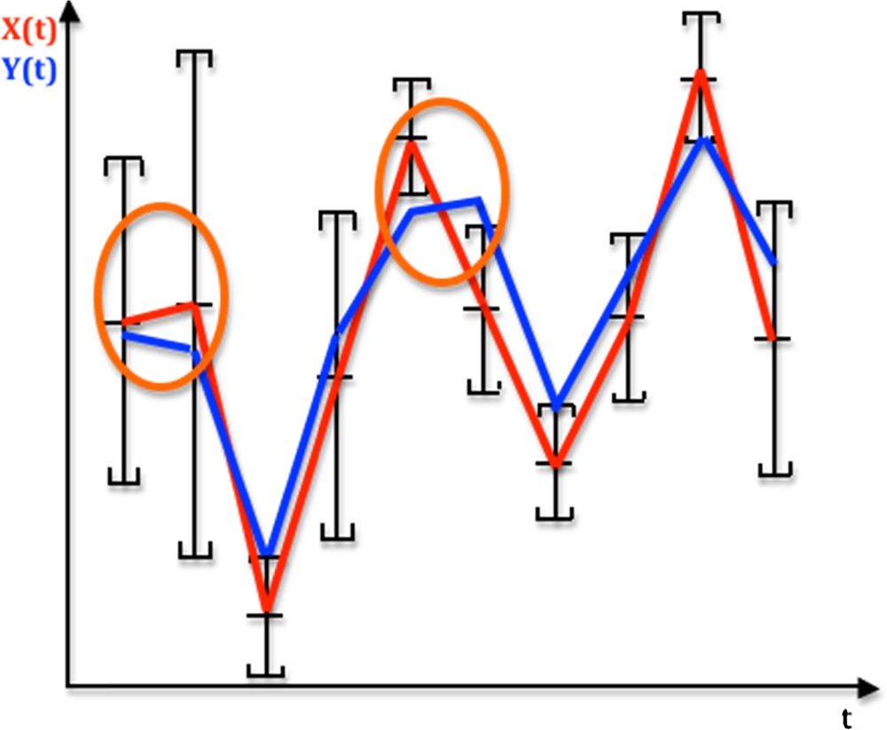
(Color online.) Temporal profiles of an observed signal X (red) and a reference signal Y (blue) over time t, indicating monotony segments between the successive averages of X, each average being the centre of the empirical 95% confidence interval of a distribution of errors on X supposed to be symmetrical. If it is supposed to be uniform, the weighted monotony signature of X is equal to (0.4,1,0,0,1,1,0,0,1). Monotony intervals circled in orange correspond to the difference between X and Y monotonies.

We can decide that the monotony signature of the observed X profile is significantly different from the Y reference profile (Fig. 1), after testing the similarity of these signatures due to a common causality between X and Y (hypothesis H1) against a random choice of the values of the successive sgnX_i's (hypothesis H0), by using, when sgn_iY = −1, the probability P__i decreasing from a value taken on the support in (denoted above S(f_i)) of the distribution f_i of X_i to a value of X_i ₊ ₁ on S(f_i ₊ ₁) (cf. Fig. 2 for i = 1):

P_{- i} = P (\{X_{i + 1} < X_{i}\}) = P (\cup_{ξ \in S (f_{i})} (\{X_{i} = ξ\} \cap \{X_{i + 1} < ξ\})) = \int s {}_{(f_{i})}f_{i} (ξ) F_{i + 1} (ξ) d ξ

(3)

where F_i+1 is the cumulative distribution function of X_i ₊ ₁.

Fig. 2
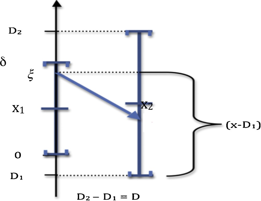
(Color online.) Calculation of the probability P_ of negative monotony, where [0,δ] (resp. [D₁,D₂]) and x₁ (resp. X₂) denote the interval and the mean of the uniform law of X₁ (resp. X₂).

The sequence of the probabilities {P__i}_i ₌ _1,…,n–1 of decay of X on its ith monotony interval is called the weighted monotony signature of X.

2.2 Gaussian errors

Proposition 1 In the Gaussian case, where the distribution of X_i is N(x_i,σ_i), we have:

P_{- i} = \int_{0}^{1} exp [(- {(g_{i} (z) - b)}^{2} + a^{2} g {(z)}^{2}) / 2 a^{2}] / a d z

(4)

where a = σ_i/σ_i+1, b = (x_i–x_i+1)/σ_i ₊ ₁ and g_i = F_i⁻¹.

Proof 1 If the density distribution of errors is Gaussian, the formula (3) becomes (by neglecting the index i):

P_ = ʃ_IR f(ξ) F(aξ + b) dξ,

where f (resp. F) is the distribution (resp. cumulative distribution) function of the standard Gaussian law N(0,1), a = σ₁/σ₂ and b = (μ₁ – μ₂)/σ₂. By changing the integration variable ξ in z = F(ax + b), we have:

dz = af(aξ + b) dξ and ξ = (g(z) – b)/a,

where g = F⁻¹. Then we can write P_ under the following formula:

P_= \int_{0}^{1} [f ((g (z) - b) / a) / a f (g (z))] d z = \int_{0}^{1} exp [(- {(g (z) - b)}^{2} + a^{2} g {(z)}^{2}) / 2 a^{2}] / a d z = \int_{0}^{1} exp ((b (2 g (z) - b)) / 2) d z if a = 1

Because the cumulative distribution functions of the uniform law on [–2σ, 2σ] and of the Gaussian law N(0,σ) are very close (cf. Fig. 3, right), the results concerning the calculations of P_ are similar. Then, in any case of errors, we have chosen uniformly 100 couples of values (x_i,x_i ₊ ₁)_i ₌ _1,…,100 in [0,10]². Then, we simulated 100 samples of 100 couples of values (ξ_ik,ξ_(i ₊ _1)k)_k ₌ _1,…,100 by using 100 couples of Gaussian distributions {N(x_i,1), N(x_i ₊ ₁,1)}_i ₌ _1,…,100, and we calculated the difference Δ_i between the probability P__i calculated from the integral formula (1) and the empirical frequency P__i* obtained from the observation of the events {ξ_ik > ξ _(i ₊ _1)k}_k ₌ _1,…,100. The result is given in Fig. 3 (left), showing as expected that the empirical distribution f_Δ* of the random variable Δ_i = P__i – P__i* is asymptotically (in sample size) Gaussian N(0,1).

Fig. 3
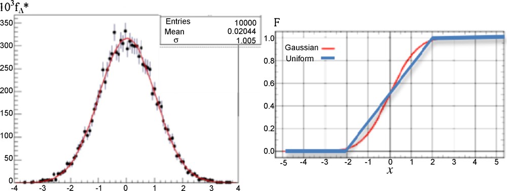
(Color online.) Left: empirical distribution f_Δ* of the random variable Δ = P_–P_*, asymptotically (in sample size) Gaussian N(0,1) (red curve). Right: theoretical cumulative function F of the uniform (blue) and Gaussian (red) distributions of errors.

2.3 Uniform errors

Proposition 2 In the uniform case, let denote by [0,δ] (resp. [D₁,D₂]) and x₁ (resp. x₂) the interval and the mean of the uniform law of X₁ (resp. X₂). Then, there are six different configurations (cf. Fig. 4):

Fig. 4
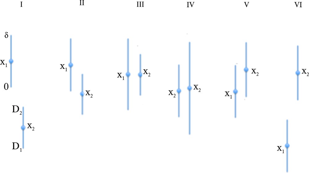
(Color online.) The six different configurations of X₁ and X₂ supports in the case of the uniform distributions of errors.

1) D₁ < 0 ≤ δ ≤ D₂, then P_ = [(δ – D₁)² – D₁²]/2δD = δ/2D – D₁/D I

2) D₁ < 0 ≤ D₂ < δ, then P_ = 1 – D₂²/2δD II

(5)

4) 0 ≤ D₁ ≤ D₂ < δ, then P_ = 1-(D₂²-D₁²)/2δD = (2δ-(D₂ + D₁))/2δ IV

5) D₁ > δ, then P_ = 0 V

6) D₂ < 0, then P_ = 1 VI

Proof 2 In the uniform case, the formula (3) becomes:

P_= \int_{\sup (0, D 1)}^{inf (δ, D 2)} f (ξ) F (ξ) d ξ,

Hence, we have:

inf(δ,D2)

If D_{2} \geq δ, P_= \int_{\sup (0, D 1)}^{inf (δ, D 2)} (ξ - D_{1}) d ξ / δ D

inf(δ,D2)

If D_{2} < δ, P_= 1 - \int_{\sup (0, D 1)}^{inf (δ, D 2)} d ξ / δ D

Then, by considering all the possibilities of values of the extrema inf(δ,D₂) and sup(0,D₁), we get the six different formulas (5) (cf. Fig. 4) ■

3 A statistical test of monotony

We will suppose in the following that the distribution function of X_i is uniform on [a_i1,a_i2] and that X is a stochastic process with independent components and increments. In Fig. 1, the probability P_ of decay of X is equal to 0.4 for the first interval of monotony and 1 for the fifth (both circled in orange). P_ equals also 1 for the second, sixth and ninth intervals, and 0 for the third, fourth, seventh and eighth ones. Let us denote by P(η) the probability of having η differences between the signs of monotony of observed X(t) and reference Y(t) signals. We call H0 the hypothesis saying that monotony signatures of X and Y are similar by chance with independency between X and Y, the probabilistic structure being defined by the empirical estimates of their distributions and the independency of the components and increments of X.

Then, if η = 2, the probability P(2) under the hypothesis H0 equals:

(6)

where P_≠i is the probability that the monotonies of X and Y are different on the ith interval:

• in the case where sgnY is deterministic, P_≠i = P__i if sgnY_i = +1 and P_≠i = 1–P__i if sgnY_i = –1;
• in the case where sgnY is random and independent of sgnX: P_≠i = P__i(X)(1–P__i(Y)) + (1–P__i(X))P__i(Y), where P__i(X) denotes the probability that X decreases on its ith monotony interval.

In the case of Fig. 1, we have, by supposing the successive monotony signs of Y known with a certainty of 3/4:

(7)

We can therefore consider that the probability of rejecting falsely the hypothesis that monotony similarity, except for η = 2 intervals, is due to chance with independency between X and Y is less than 5%. This test is not as powerful as a correlation test, but it is interesting in the case of a low number of longitudinal observations in which signal amplitude is not pertinent compared to monotony, when the variance of the empirical correlation with a reference signal is important. Easy calculations above require that reference Y and observed signal X are known at the same instants of observation and random process X(t) has independent components and increments. The cause of rejecting the hypothesis of similarity with independency between X and Y is the presence of a link between successive values of the observed and reference signals.

4 Biomedical applications

We will give in the following simple illustrative examples where monotony signature is pertinent.

4.1 Genetic events localization

Fig. 5 below gives the localization X (resp. Y) of the physiologic crossing-overs along chromosome 3 for human females, with the blue curve in Fig. 5 (resp. males, with red bars) [4]. By comparing the two monotony signatures as given, we reject the hypothesis that female and male crossing-overs have similar localization by chance with independency between X and Y (P < 10⁻⁷), which is in favor of the existence of the same frailty domains along the male and female chromosome, explaining the frequency of crossing-over co-occurrences.

Fig. 5
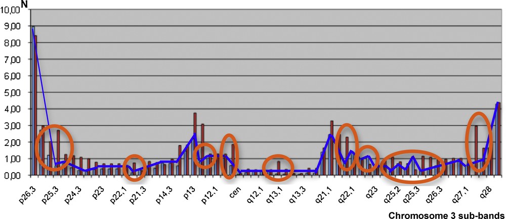
(Color online.) Crossing-over numbers N (male red bars and female blue curve) along the human chromosome 3 (12/63 monotonic discrepancies encircled by orange ellipses).

4.2 Individual choices and collective consciousness

During successive sessions of choice, participants belonging to a defined group are choosing one picture from an “absurd questionnaire” consisting of 50 pairs of pictures, in each of which one picture has to be chosen [5]. The results given in Fig. 6 are used to search for evidence in favor of the influence of group dynamics on individual choices of the pictures proposed in the questionnaire. The swaps between the two pictures of a pair, measured for each pair of pictures between the initial choice (called A choice) across sessions could be interpreted as a manifestation of group dynamics: for instance, the “honeymoon” (dependence on the leader) and the successive “fight-flight” (reaction against the dependence on the leader) attitudes could be represented by a greater number of group dynamics swaps (further away from pure randomness). It seems intuitive that an increase of simultaneous swaps could be linked to an increased group activity or group dynamics event. Statistics carried out on the totality of swaps A→B or B→A evidenced a significant increase in the swap numbers between S01/S02 and S02/S03 session transitions, and between S03/S04 and S04/S05 session transitions, incompatible with a random fluctuation. In other words, the number of changes in choices increased significantly between the 1st and the 3rd sessions, and then remained essentially constant until the end of the training, except between the 3rd and the 5th sessions. During session S04, the number X of A→B swaps and Y of B→A swaps showed similar fluctuations close to significance against similarity obtained by chance with independency between X and Y (P = 0.6), while there is no significant change in the evolution of the sum X + Y. This is consistent with the existence of a collective unconscious behavior.

Fig. 6
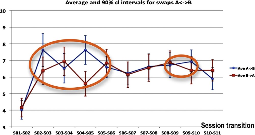
(Color online.) Group dynamics-driven swaps from picture A to B and from picture B to A, occurring over time between 11 consecutive sessions for each of 50 pairs of pictures, for the two types of swaps (A to B and B to A). We see inside orange ellipses the localization of discrepancies between the monotony of the curves relative to A→B and B→A swap numbers.

4.3 Actimetry

After 25 days of observation of a person at home [6–8], we get the results given in Fig. 7 corresponding to his/her staying in the different rooms of a smart flat in which different sensors recorded his/her activity at home. They allow us to calculate different temporal profiles assigning the observed person in different clusters corresponding to a normal or a pathologic behavior. Alarms can be triggered when passing from a normal type of nychthemeral activity to a pathologic one. For example, in a degenerative neural pathology like Alzheimer's disease, we can observe an abnormal activity in the same room, called perseveration, which is a pathologic repetition of actions in general already successful (“errare humanum est, perseverare diabolicum”) [9]. We model this phenomenon of persistence in a pathologic activity by setting atypical extended occupancy periods in a room or by performing repetitively a specific daily routine, in comparison to more standard scenarios encountered in everyday life.

Fig. 7
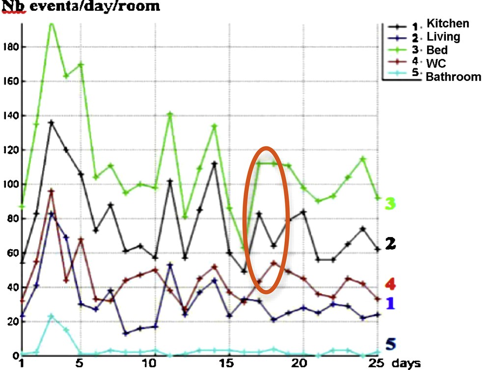
(Color online.) Evolution during the nychthemeron (day/night 24-h interval) of the number of entrances in room, for different rooms, during 25 successive days. We see in orange the localization of the monotony dissimilarities between curves No. 3 (number of entrances in bedroom) and No. 4 (number of entrances in the toilets).

A way to compare different temporal evolutions of room occupancies is to follow the evolution in time of the number of events of entrance in room, for different rooms and 25 successive days. The fluidity of the activity can be related to the number of entrances in connected rooms like the bedroom and the toilets, because a decorrelation between these numbers could sign a stereotyped activity by repeating for example pathological entrances in the toilets or non-entrances from the bedroom (e.g., in case of anuria, nocturia, or pollakiuria). The data in Fig. 7 show that only three discrepancies within a period of 25 days allow us to reject a similarity between entrance activities No. 3 and No. 4 by chance, with independency of these activities (P = 2 × 10⁻⁷), the same monotony signature for connected rooms being then the sign of a normal behavior.

4.4 Microtubule morphogenesis

In [9,10], the authors recall that weightlessness is known to affect cellular functions by as yet undetermined processes, but with a role of the cytoskeleton and microtubules, which behave as a complex system that self-organizes by a combination of reaction, diffusion, collective transport and self-organization of any present colloidal particles [9]. This self-organization does not occur when samples are exposed to a brief early period of weightlessness [10]. During both space-flight and ground-based (clino-rotation) experiments on the effect of weightlessness on the transport and segregation of colloidal particles, a significant difference between the velocity of colloidal particle beads has been observed (Fig. 8), as well as the rejection of the similarity by chance with independency between gravity and non-gravity monotony signatures during the evolution of the microtubule organization in embryonic cells (P = 3 × 10⁻⁵). This suggests, depending on factors such as cell and embryo shapes, that major biological functions associated with microtubule-driven particle transport and self-organization might be strongly perturbed in velocity amplitude, but not in sequencing, by weightlessness.

Fig. 8
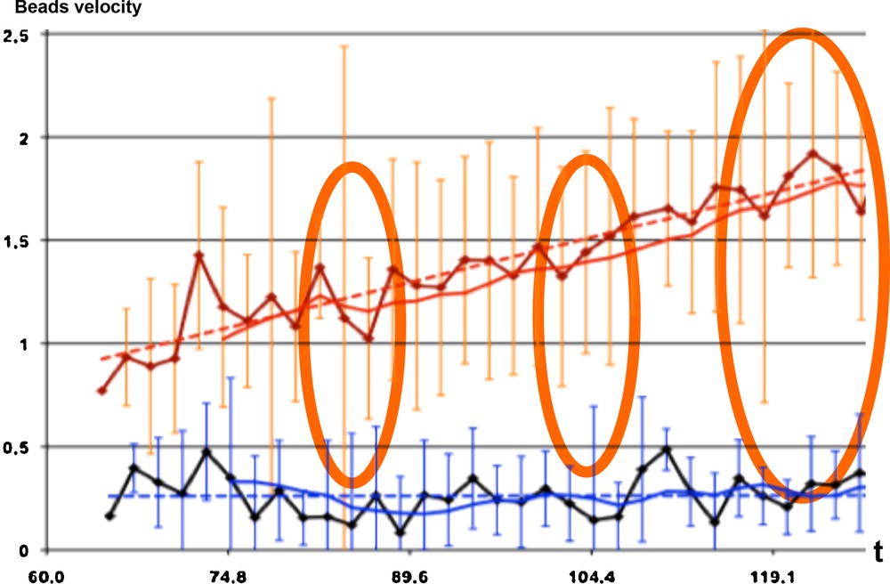
(Color online.) Evolution during 60 s of the observed number of beads in the cell preparation, showing 4/30 discrepancies (orange ellipses) between the bead numbers observed under a gravity field (1G for the red curves) and in the absence of gravity (black and blue curves).

5 Conclusion

The stochastic signature of monotony and the associated statistical test of similarity of monotony allow us to manage situations in which two signals have to be compared, not in amplitude, but only through the succession of their monotony intervals. Numerous situations in which this approach can be used exist in biology, and we have selected four cases in biomedicine, in which the present tool seems to be pertinent.

If there exists an empirical correlation between two successive increments, then the test must be done with a reference signature provided with this correlation structure estimated from the empirical law. It is the case if the process is observed through a longitudinal sampling of individual histories, even if the process has independent components. More, if the components are not independent, but if it is possible to calculate the joint empirical distribution of the signs of monotony signature for each individual history, provided it makes sense at the observation level (time sampling allowing the estimation of the non-Markovian dependence of the increments), and if we know the distribution of the reference signature, then the test to be used is an identity test between reference and empirical distributions. This situation will be studied in a future article.

Disclosure of interest

The authors declare that they have no competing interest.

Acknowledgements

We are very indebted to Yannick Kergosien for his helpful suggestions and exciting discussions.