

1 Introduction
In recent years, it has become possible to make simultaneous measurements of the expression levels of tens of thousands of genes using the so-called microarray technology. Through various microarray experiments, scientists try to answer various basic biological questions ranging from understanding some aspect of the cell cycle mechanism of a given organism to the identification of individual genes involved in some biochemical pathway related to some biological function or some disease of interest.
In this article, we discuss statistical modelling of data from high-density oligonucleotide arrays of the type manufactured by Affymetrix. The point of view we adopt is that statistical methods can and should be used in order to achieve a better understanding of experimental data. Although statistical methods can be useful at all the stages of a typical microarray experiment (experimental design, image analysis and artefact detection, normalization, calculation of gene expression, making comparisons between arrays, dimension reduction, clustering, etc.), we will only discuss the fundamental problem of estimating the expression index (cf. [1,2]).
The article is organized as follows. In Section 2, we describe how the data arise in some detail. The bivariate Li–Wong model (cf. [3,4]) is presented in Section 3. This model is used in Section 4 to provide maximum likelihood estimates of various parameters. A new way of reducing the model into a univariate one and the resulting estimates are discussed in Section 5. Comparisons between these two estimates as well as others are discussed in the discussion section.
The main conclusion of the article is that the new estimates seem to be better than previously established ones.
2 The nature of the data
First we take a look at some of the features of oligonucleotide-based microarrays. A single array (1.28 cm×1.28 cm) can contain probe sets for tens of thousands of genes and ESTs. Every probe set consists of 10–20 probe pairs. Every probe pair contains a perfect match (PM) probe and a mismatch probe (MM). The perfect match probe is a small DNA subsequence (25 bases long), which is assumed to be specific for a particular gene, the expression of which we want to measure. The mismatch probe is identical to the perfect match probe, except for the base in the middle (13th) position.
The oligonucleotides in the probes are typically chosen from the so-called 3 prime end of the gene, but have been until recently unknown to the user. The expression level of the gene has to be inferred from the amount of hybridisation of the PM and MM probes. The latter are measured using a scanner, which is sensible to the fluorescence intensities of the probes. Up to now, expression indices have been based on PM–MM differences at the probe level. Contrary to what one expects, such differences are often negative. A trial study reveals that although very few probe sets will only have negative differences, a vast majority will have some. In fact, the median number of negative probes per probe set is around 8 (out of a total of 20). In many cases, the overall average of these differences for a probe set will be negative. Since this means that the corresponding gene has negative expression, it is obvious that such an average difference cannot be used. Various conditions are often imposed to prevent this from happening. These include using PM values only (cf. [1,2,5]), excluding probe pairs with negative differences, using PM−c MM with some suitably chosen constant c (cf. [6]), treating negative differences as missing data and using imputation, etc. All these methods suffer from drawbacks such as being ad hoc, being inconsistent in that not all probe pairs are used in the same way, etc. This obscures the analysis.
At the most basic level, the data is in the form of pixel intensities (36 pixels/cell for the Mu11k mouse chip) for the individual probe cells. It goes without saying that one can (and should) try to model the data already at this level using ideas from statistical image analysis. In these notes, however, we will only consider models on the next level, namely that of PM and MM intensities. Another issue that we will not discuss here is that of background calculation and subtraction.
3 The model
The basic idea behind the Li–Wong model (cf. [3,4]) is that the PM intensities are expected to be higher than the MM intensities. One can thus assume the following model: (1)
All these quantities are assumed to be non-negative. Moreover in order to avoid ‘unidentifiability’, we impose some additional conditions like ∑jφj2=J. Although this model was introduced in [3], the authors have only treated the reduced case
| (2) |
The authors of [7] use (1) explicitly, but assume that the PM and MM values are independent; so their model describes the marginal distributions. We propose to augment the model so as to take into account the empirically observed correlation between PM and MM, which is usually rather high. For example, the average correlation coefficient for 30 probe sets was 0.77 with a standard deviation of 0.14. The maximum value was 0.94 and the minimum 0.36 (cf. Fig. 1).
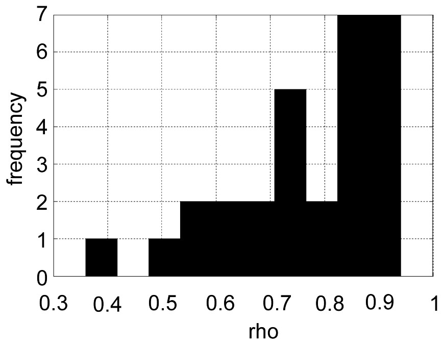
Shows the distribution of the PM/MM correlation for 30 probe sets (ρ on the x-axis and the frequency on the y-axis).
The rationale for this is that the probe pairs corresponding to the same gene are scattered all over the array, while the two components of the same probe are always adjacent to each other. More precisely, we assume that the error terms in (1) follow a bivariate normal distribution according to:
| (3) |
How do we know that such a model fits the data? It is possible to examine the adequacy of the model by using the residuals to measure the lack of fit. The reader will find more information about this at the end of the next section.
4 The estimates
Given data (Pij,Mij), we can find parameter estimates using the maximum-likelihood method. The likelihood function has the form:
These formulas have to be understood as steps in an iterative procedure that will lead to the final estimates. Nonetheless they are quite useful when it comes to deriving various properties. It is thus easy to see that the estimate, of the expression index is unbiased, i.e. that . The usual expression index (the average difference or advocated by Affymetrix) lacks this property, as is seen by the following argument. In terms of the Li and Wong model, we have . From Steiner's theorem, we know that so , i.e. is unbiased.
To obtain non-parametric confidence intervals for the expression level, we propose the following bootstrap method. First, estimate the parameters using the above maximum likelihood estimates; then, estimate the means:
| (5) |
Notice also that the common PM/MM variance can be (ML) estimated by:
5 Reduced models
As mentioned earlier, the Li–Wong model has, until now, been only used in its reduced form (2). This has the advantage of being a much simpler model than the full one. This reduced model has been implemented in dChip (one of the most popular tools for analysing this type of data). Other ways to get reduced models have also been investigated: using PM only values or the average difference. It is possible to formulate a reduced version of the Li–Wong model along the lines proposed in [6], i.e. by considering Pij−cMij for some suitable value of c.
In what follows, we present a new way of reducing the full model. The rationale of this method is that the MM values can, in a sense, be considered as containing help information only. One way to use this help information is to condition on it, i.e. to consider the conditional distribution of the PM values given the MM values. Under the assumption that the bivariate values are normal, the conditional distribution is also normal according to (cf. [8]):
Again, maximum likelihood estimates of the parameters can be based on this model. The resulting estimate of the expression level is:
It is rather easy to verify that this estimate is unbiased.
6 Discussion
We have thus seen that using the Li–Wong model as a basis, one has the choice of using either the full bivariate model or some reduced univariate version. To make a rational decision as to the choice of a model, one can use both theoretical and empirical criteria as is done in [9]. One such criterion is unbiasedness. But perhaps the most natural of these criteria is the variance, i.e. preferring an estimate with a low variance over one with a large variance. Simple calculations show that according to this criterion the best model is the full bivariate model followed by the conditional and the reduced models in that order (cf. the Appendix). The comparison with the average difference is, however, not straightforward since that estimate has to be transformed to become unbiased. The transformed average difference has the largest variance of all reduced models.
A quite different way of comparing models is to use special experiments where known amounts of mRNA are used. Such data will become more available in the future.
It is interesting that the gene expression estimate based on the conditional model is of the type proposed by [6], i.e. of the form Pij−cMij. In this estimate, the constant c is simply taken as ρ, the correlation coefficient. The conditional estimate has one additional nice feature, namely that it is a weighted average of Pij−ρMij differences. Probe pairs with higher sensitivity (measured by αj(1−ρ)+φj) are given a higher weight. The special cases ρ=0 and ρ=1 give the PM-only case and the reduced Li–Wong model respectively. To gain insight as to why ρ is a good choice of constant in the approach used in [6], one can argue as follows. The variance of each term Pij−cMij is simply σ2(1+c2−2ρc) and is minimized when c=ρ.
To conclude, we have argued that, in the sense of unbiased estimates having low variance, the best estimate is simply the one based on the full bivariate model. Should one choose to use a univariate reduced model, then the estimate based on the conditional distribution is the next best choice. The latter has many desirable properties and for probe sets having high correlation coefficients, it is quite similar to the estimate based on the Li–Wong reduced model.
Appendix
In this appendix we give the variances of the different estimators mentioned in the article.
- 1. The estimate based on the full model:
(6) - 2. The estimate based on the conditional model
(7) - 3. The estimate based on the reduced Li–Wong model
(8) - 4. The transformed average difference
(9)