


 CC-BY 4.0
1. Introduction
Human-induced pressures are at the root of the ongoing environmental crisis (Ceballos, Ehrlich, et al., 2015), which results in strong biodiversity losses in many taxa, including birds (BirdLife International, 2022; Inger et al., 2015), insects (Hallmann et al., 2017), mammals (Ceballos and Ehrlich, 2002) and plants (Vellend et al., 2017; Jandt et al., 2022), and also has consequences for ecosystem functioning (Biesmeijer et al., 2006; Martin et al., 2019). To deal with this situation, policymakers try to provide guidelines to take action against the current biodiversity crisis. For instance, the recent Kunming-Montreal Global Biodiversity Framework sets four strategic goals and 23 targets to mitigate biodiversity loss by 2050 (CBD, 2022). In particular, the first set of targets aims at reducing threats to biodiversity, with Target 4 specifically highlighting the need to “ensure urgent management actions to halt human-induced extinction of known threatened species and for the recovery and conservation of species, in particular threatened species, [and] to significantly reduce extinction risk”. This requires the identification of species whose populations are declining and careful monitoring of the conservation status of threatened species.
To fulfill these goals, there is an urgent need to reinforce our knowledge of the current state and dynamics of biodiversity, as well as to develop reliable indicators that quantify and qualify trajectories in biodiversity changes. These indicators must encapsulate complex phenomena in a simple, understandable, and non-ambiguous way, be easy to communicate, ecologically relevant, sensitive to changes, and possess suitable mathematical properties, especially high precision and absence of bias (Gregory Richardet al., 2005; Van Strien et al., 2012). In view of these characteristics, estimated temporal trends in species abundance or occurrence have been proposed as relevant indicators at the population scale (Pereira et al., 2013). However, many methodological choices in the production of these trends remain arbitrary and vary significantly across observatories, which can lead to inconsistencies and hinder their comparability (Dornelas et al., 2013; Toszogyova et al., 2024).
The estimation of temporal trends relies on long-term monitoring of species abundance or occurrence. Such data are difficult to collect, especially at large spatial scales, because of the required sampling effort and associated costs. One way to tackle this issue is to use citizen-based monitoring programs, which rely on non-professional volunteers to collect biodiversity data using standardized protocols. This approach has multiple benefits, including lowering the costs (Levrel et al., 2010; Theobald et al., 2015), expanding the spatial coverage, while also developing public engagement regarding conservation matters (Deguines et al., 2020; Pocock et al., 2018).
Although concerns have been raised regarding the reliability of citizen-based data, with a focus on knowledge gaps between participants and variations in sampling effort over time and space (Dickinson et al., 2010), there are now recommendations on the most suitable monitoring frameworks for temporal trend estimation (Pescott, Walker, et al., 2015) and on statistical tools that facilitate data analysis while possibly accounting for those biases (Pannekoek and Van Strien, 2005). This may explain the success of such programs, measured by the number of scientific studies derived from citizen science (Cooper et al., 2014; Fraisl, Hager, et al., 2022) as well as the development of citizen-based spatial and temporal indicators (e.g., UK plant atlas or European Common Bird Indicator) that are used by local and international institutions (Chandler et al., 2017; Fraisl, Campbell, et al., 2020).
In France, Vigie-Nature is a citizen science program that offers multiple schemes for volunteers to observe and monitor biodiversity, depending on their knowledge and taxa of interest (http://www.vigienature.fr; Julliard, 2017). The French Breeding Bird Survey (called STOC, the French acronym for Suivi Temporel des Oiseaux Communs), which focuses on common bird monitoring by skilled volunteer ornithologists, is one of the oldest schemes (created in 1989). It is already used both nationally and across Europe to inform on trends in bird populations, depending on habitat specialization (Fontaine et al., 2020). Vigie-flore is a more recent scheme that started in 2009, involving a large community of skilled volunteer botanists to record the presence of vascular plants. Although no population trends have yet been estimated from this monitoring program, it has been used to assess the effects of climate change on plant community composition (Martin et al., 2019).
The production of annual population trends is expected by funding institutions, NGOs involved in biodiversity conservation, and participants. Furthermore, population abundances and their trends are part of the Essential Biodiversity Variables (EBV) used to set IUCN conservation statuses; they should hence be produced using open, robust and reproducible statistical methodologies. Some tools already exist for producing population trends based on count data, like the one in (Pannekoek and Van Strien, 2005), and are commonly used for taxa such as birds (see the Pan-European Common Bird Monitoring Scheme (PECBMS) [https://pecbms.info]). However, they are not yet suitable for analyzing occurrence data, such as those obtained from plant monitoring in Vigie-flore. Beyond the choice of relevant statistical approaches, producing population trends from citizen science data involves fundamental steps of data processing that need to be standardized and made available.
Here, we present the analysis pipeline we developed to estimate population trends, handling various data types (such as counts and presence/absence), and taking into account the protocol specificities of each monitoring scheme. We also present the resulting species population trends for 148 common bird and 181 common plant species in France, based on data collected through the STOC and Vigie-flore monitoring schemes over the past 35 and 15 years, respectively. We further introduce new criteria for trend characterization and classification. Finally, we provide new graphical representations of results to improve outreach, from understanding uncertainty to non-linearity.
2. Methods
2.1. Data
2.1.1. Bird abundance monitoring scheme
Bird abundance data were produced by the STOC, a citizen science scheme that has been monitoring common birds in France since 1989. This program relies on a network of skilled volunteer ornithologists who are assigned a 2 × 2 km square sampled from a systematic grid. Each square contains 10 counting points that are representative of the habitats found within the square. Each year, volunteers record all bird individuals seen or heard during five minutes at each of these counting points. Each year, there are two recording sessions during the breeding period, separated by four to six weeks. The early session is held before May 8th to sample the early singing birds, and the late session is held after May 8th, to sample the late migrants. To record only birds that are actual breeders on the monitoring sites, the migratory species that are still on their way to Northern Europe at that time (yellow wagtail Motacilla flava, whinchat Saxicola rubetra, meadow pipit Anthus pratensis, northern wheatear Oenanthe oenanthe, willow warbler Phylloscopus trochilus and fieldfare Turdus pilaris) are excluded from the dataset of the first session. Recording sessions must occur between one and four hours after sunrise and must be repeated around the same dates every year.
The STOC protocol changed in 2001: before this date, squares were chosen by volunteers. Since 2001, they have been randomly assigned within a 10 km buffer around a location provided by volunteers. This sampling design is more representative of habitats across France. Also, the number of counting points per square ranged from five to 15 before 2001, but was fixed to 10 afterwards. Finally, the number of mandatory visits per square and year increased from one to two in 2001. A full description of the protocol is available on the Vigie-Nature website [http://www.vigienature.fr]. Due to this change in protocol, we generally discarded the 1989–2000 data, except for the estimation of an historical trend (see below).
We analyzed bird counts at the year and square levels. For each year, species, and counting point, we retained the maximum number of individuals recorded over the two sessions, and then summed these values for all points within a square. This sum was used as a proxy for the species abundance in a given square and year.
As volunteers are, by definition, free to join and quit the monitoring program at any time, squares were monitored over a variable number of years. Over the 1989–2023 period of interest, 886 squares (24%) were monitored for a single year, and on average squares have been monitored for 5.9 years. For the analysis, we only retained squares that were visited for at least two years, as squares monitored for a single year are not informative for population trends. This led to a total of 21 010 visits of 2815 squares, of which 1134 visits of 184 squares occurred before the 2001 change in protocol.
We analyzed the 148 most common species, defined as species observed in at least five squares per year on average. As only presence (and abundance) data are registered by volunteers, we reconstructed absence data using the following procedure: a species observed at least one year in a square was assigned an abundance of zero for all years in which the species was not recorded, although the square was monitored.
2.1.2. Plant sampling protocol
Plant occurrence data were produced by Vigie-flore, a French citizen science program that monitors wild flora in France since 2009. This program relies on a network of skilled volunteer botanists who are randomly assigned a 1 × 1 km square sampled from a systematic grid. Each square contains eight systematically distributed 10 m2 plots, which consist of 10 contiguous quadrats of 1 m2. Each year, volunteers record all vascular plant species that are present in each quadrat. The proportion of quadrats in which a species is observed (species frequency) is used as a proxy for its abundance in each plot. The monitoring period is chosen depending on the square location: squares located in the Mediterranean biogeographical region are monitored between April 1st and May 31st; those located in continental or Atlantic regions are monitored between June and July; and squares located in areas with an elevation above 1000 meters (alpine region) are monitored between July and August. A full description of the protocol is available on the Vigie-Nature website [http://www.vigienature.fr].
For the same reasons as for the bird dataset, squares were monitored for a variable number of years: 277 squares (41.6%) were monitored for a single year, and, on average, squares were monitored for four years. For the analysis, we retained squares that were visited for more than one year, meaning 2339 visits of 388 squares.
We analyzed the 181 most common species, defined as species observed in at least ten squares per year on average. This threshold was set higher than that for birds to compensate for the lower precision of presence/absence data regarding count data. Absences were reconstructed using the same methodology as for the bird dataset.
2.1.3. Land cover data
We characterized land cover on Vigie-flore plots and STOC squares using the CORINE Land Cover (CLC) inventory (Bossard et al., 2000), which relies on visual interpretation of high-resolution satellite imagery to classify land cover into 44 classes. Four updates were made in 2000, 2006, 2012 and 2018. STOC squares and Vigie-flore plots were thus associated with the closest previous CLC update: CLC 2018 for squares and plots visited since 2018, CLC 2012 for squares and plots visited between 2012 and 2018 (excluded), and so on.
We categorized the 44 land cover classes into five broad classes: forest, agricultural, urban, water and other land cover (see Table 1). For the bird dataset, land cover was characterized through the percent cover of each of the five broad classes found in a 1 km buffer around the center of each STOC square. The percentage of agricultural cover was removed from the analysis to avoid multicollinearity in models, as all percentages sum to 100. For the plant dataset, land cover was characterized through a five-class variable corresponding to the major land cover (i.e., land cover with the largest area) found within a 5-meter buffer around the center of each Vigie-flore plot. This buffer size was chosen so that land cover could be described locally. The choice of a categorical variable is justified by the negligible number of plots with multiple land cover classes within the buffer.
Grouping of the CLC 44 land-use classes into five broad classes
| Broad classes | Original 44 classes |
|---|---|
| Forest cover | Level 3.1-Forests (3 classes) |
| Level 3.2-Shrub and/or herbaceous vegetation associations (4 classes) | |
| Agricultural cover | Level 2-Agricultural areas (11 classes) |
| Urban cover | Level 1-Artificial surfaces (11 classes) |
| Water cover | Level 4-Wetland (5 classes) |
| Level 5-Water bodies (5 classes) | |
| Other covers | Level 3.3-Open spaces with little or no vegetation (5 classes) |
2.2. Estimation of temporal trends in bird abundance or in plant probability of occurrence
2.2.1. Population trends estimation
For each species in the plant and bird datasets, we estimated a linear population trend over the entire monitoring period (2001–2023 for birds and 2009–2023 for plants), as well as a linear population trend over the last ten years (2014–2023). To do so, we fitted a generalized linear mixed model for each species, using the R package glmmTMB (Brooks et al., 2017), following previous work on similar datasets (Sauer and Link, 2011). Covariates were introduced to correct for possible biases in trend estimation, following a variable selection procedure based on Bayesian Information Criteria (Supplementary material “Variable Selection Procedure”). For the plant dataset, the only covariate retained was the observation date, in a Julian date format. For the bird dataset, the recording session was included as a three-level variable: early session, late session or both sessions. Land cover (described above) was also retained. For collinearity matters, we excluded agricultural cover. Finally, elevation was also added as a fixed effect, as well as longitude and latitude, which were both treated as 2nd order polynomial effects, and their interaction (see Table 2).
Variables included as fixed effects in the models for trend estimation
| Variables name | Type | Description | STOC | Vigie-flore |
|---|---|---|---|---|
| Year | int | Observation year | X | X |
| Forest_cover | num | Percent forest cover | X | |
| Urban_cover | num | Percent urban cover | ||
| Water_cover | num | Percent water cover | ||
| Other_cover | num | Percent other covers (excluding agricultural cover) | ||
| Longitude | num | Longitude coordinates, treated as a 2nd order polynomial | X | |
| Latitude | num | Latitude coordinates, treated as a 2nd order polynomial | ||
| Longlat | num | Interaction between longitude and latitude coordinates | ||
| Elevation | int | Elevation | ||
| Date | int | Date of observation, in a Julian date format | X | |
| Visit | char | Recording session (three categories: early session, late session, both sessions) | X |
Random effects were also introduced in those models, to take dependence among observations into account. This dependence is mostly due to repeated observations in the same squares and/or by the same volunteers. For birds, we included a random intercept for squares nested within administrative départements. For plants, we included a random intercept for plots nested within squares, as well as a random intercept for volunteers. For both datasets, we also added a random effect of plots on the slope of the year effect.
For bird abundance, we used a negative binomial distribution with a quadratic parametrization as well as a log link function, designed to handle overdispersion in count data. For plant occurrence, we used a beta-binomial distribution with a clog-log link function, designed to handle overdispersion in presence/absence data.
2.2.2. Annual variations
To estimate annual variations in bird abundance and plant occurrence, we fitted a generalized linear mixed model with similar specifications as above, but with two major changes. First, the variable year was treated as a categorical variable rather than a continuous variable. This allows for the estimation of the difference in mean abundance between each year and a reference level. This reference level is usually set to the abundance of the first year, but due to the low number of observations during the first year of both monitoring schemes, we set the reference level to the mean abundance across all years, thus avoiding convergence issues. Second, as year is treated as a categorical variable, the models did not include random slopes for the year effect across squares/plots.
For visualization and communication purposes, we smoothed annual variations by fitting a generalized additive mixed model (GAMM), using the R package mgcv (Wood, 2017). Following (Fewster et al., 2000), the number of knots k was set to 30% of the time series, thus authorizing a changepoint every three years on average. As smoothing was used for illustrative purposes, we simplified the model specifications by removing random slopes. Also, due to restrictions on implemented distribution laws, we used a quasi-binomial distribution law to model plant occurrences, which also accounts for overdispersion in presence/absence data.
2.2.3. Historical trends
For each species in the bird dataset, we also estimated a linear population trend over the monitoring period that covers both protocols (1989–2023), thus adding historical data collected with the 1989–2001 protocol. Due to changes in protocol and a smaller number of observations before 2001, we simplified the model calibrated on the 2001–2023 period and used different covariates from those described above. First, proportions of water cover and other covers were removed from the covariates. Because the number of monitoring points was variable before 2001, we included it as a covariate in the model. We used the log number of monitoring points to keep proportionality between the number of points and abundance despite the log link function. To account for differences in protocols before and after 2001, we added the corresponding two-class variable as a fixed effect. Finally, recording sessions in the early protocol were not repeated twice, and no information on the timing of the single session was available (early or late session in the description of the bird monitoring protocol). To incorporate this information into the model nonetheless, we randomly assigned a timing for the recording session of each site visited before 2001 (early or late session, both with probability 0.5). This timing of sessions was fixed across the years. Finally, random effects were the same as above.
2.2.4. Uncertainty curves
To better communicate on uncertainty, we relied on (Pescott, Stroh, et al., 2022) who suggest the use of ensemble lines to represent a range of possible trajectories that are compatible with medium-term and short-term trends. For each species s, an ensemble line was built using the following procedure:
- Relative abundance means $\beta _{s}= ({\beta }_{s}^{1},{\beta }_{s}^{2},\ldots ,{\beta }_{s}^{n})$ and standard errors $se_{s}=({se}_{s}^{1},{se}_{s}^{2},\ldots ,{se}_{s}^{n})$ associated with each year i = {1,…,n} were extracted from annual variation models;
- We drew 100 simulated sets of yearly relative abundance estimates $X_{j,s}=({x}_{j,s}^{1},{x}_{j,s}^{2},\ldots ,{x}_{j,s}^{n})$, j = {1,…,100} from a normal distribution with the following parametrization: Xj,s ∼ N(𝛽s,ses);
- For each simulated set of estimates, a linear regression was fitted;
- Intercepts and slopes were then extracted from each of these regressions to draw a line ensemble that shows 100 possible trajectories.
2.2.5. Trends classification
For each species s, the estimated temporal trends in abundance/occurrence ${\beta }_{s}^{\mathrm{year}}$ were converted to growth rates, as follows: $GR_{s}=\exp ({\beta }_{s}^{\mathrm{year}})$. The standard errors associated with the trend estimates, ${se}_{s}^{\mathrm{year}}$, were used to infer the lower $({GR}_{s}^{\mathrm{inf}})$ and upper bounds $({GR}_{s}^{\mathrm{sup}})$ of the growth rate confidence interval:
| \begin {eqnarray*} {GR}_{s}^{\mathrm {inf}} &=&\exp ({\beta }_{s}^{\mathrm {year}}-1.96\times {se}_{s}^{\mathrm {year}});\\ {GR}_{s}^{\mathrm {sup}} &=&\exp ({\beta }_{s}^{\mathrm {year}}+1.96\times {se}_{s}^{\mathrm {year}}). \end {eqnarray*} |
Therefore, we used as lower (resp. upper) limits of our classification scheme, growth rates that matched a decline (resp. increase) of more than 30% in ten years, as lower (resp. upper) limits of our classification scheme. That is: GRlower_lim = 0.961 and GRupper_lim = 1.030. This yielded the exclusive categories that can be found in Figure 1.
Linear-trend classification depending on estimated growth rates. (a) Strong increase: the lower bound of the confidence interval is larger than the upper limit ($GR_{s}^{\mathrm{inf}}>GR_{{\mathrm{upper}\mathop{\_}\lim }}$); (b) Moderate to strong increase: the lower bound of the confidence interval is larger than 1 (significant increase) and the growth rate is larger than the upper limit ($1<GR_{s}^{\mathrm{inf}}<GR_{\mathrm{upper}\mathop{\_}{\lim }}$ and GRs > GRupper_lim); (c) Moderate increase: the lower limit of the confidence interval is larger than 1 (significant increase) and the upper bound of the confidence interval is smaller than the upper limit ($1<GR_{s}^{\mathrm{inf}}$ and $GR_{s}^{\mathrm{sup}}< GR_{\mathrm{upper}\mathop{\_}{\lim }}$); (d) Stable: the confidence interval encloses 1 (no significant trend) and is included within the interval [GRlower_lim; GRupper_lim]; (e) Moderate decline: the upper bound of the confidence interval is smaller than 1 (significant decline) and the lower bound of the confidence interval is larger than the lower limit; (f) Moderate to strong decline: the upper bound of the confidence interval is smaller than 1 (significant decline) and the growth rate is smaller than the lower limit (GRlower_lim > GRs and $GR_s^{\mathrm{sup}}<1$); (g) Strong decline: the upper bound of the confidence interval is smaller than the lower limit ($GR_{s}^{\mathrm{sup}}<GR_{\mathrm{lower}\mathop{\_}\mathrm{lim}}$); (h) Uncertain: the confidence interval encloses 1 (no significant trend) and encloses either GRlower_lim or GRupper_lim.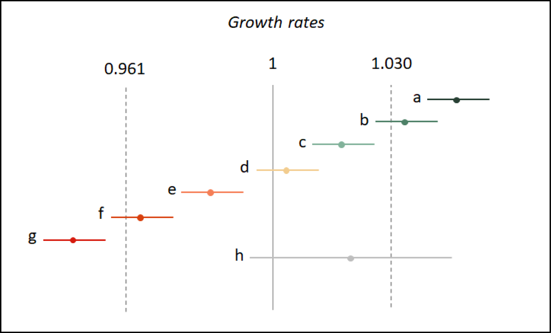
2.2.6. Population trends within habitat specialization groups
To better understand variations in species trends, we examined population trends within habitat specialization categories, sensu (Jiguet et al., 2012). We distinguished trends in generalist, rural specialist, farmland specialist, urban specialist, and other common species, hereafter referred to as “others” (Tables 3 and 4; Supplementary material “Habitat Specialization”).
Partitioning of bird long-term trends (2001–2023) within the different habitat specialization categories
| Generalists | Farmland specialists | Forest specialists | Urban specialists | Other species | |
|---|---|---|---|---|---|
| Strong increase | 7.1% (1) | 0% | 4.2% (1) | 7.7% (1) | 12.7% (9) |
| Moderate to strong increase | 0% | 0% | 4.2% (1) | 0% | 7% (5) |
| Moderate increase | 21.4% (3) | 16.7% (4) | 25% (6) | 30.8% (4) | 11.3% (8) |
| Stable | 50% (7) | 37.5% (9) | 16.7% (4) | 7.7% (1) | 23.9% (17) |
| Moderate decline | 21.4% (3) | 20.8% (5) | 41.7% (10) | 30.8% (4) | 11.3% (8) |
| Moderate to strong decline | 0% | 8.3% (2) | 4.2% (1) | 7.7% (1) | 7% (5) |
| Strong decline | 0% | 12.5% (3) | 4.2% (1) | 15.4% (2) | 1.4% (1) |
| Uncertain | 0% | 4.2% (1) | 0% | 0% | 25.4% (18) |
Partitioning of the short-term trends (2014–2023) within the different habitat specialization categories
| Generalists | Farmland specialists | Forest specialists | Urban specialists | Other species | |
|---|---|---|---|---|---|
| Strong increase | 7.1% (1) | 12.5% (3) | 8.7% (2) | 15.4% (2) | 19.4% (14) |
| Moderate to strong increase | 0% | 4.2% (1) | 8.7% (2) | 15.4% (2) | 11.1% (8) |
| Moderate increase | 35.7% (5) | 12.5% (3) | 20.9% (5) | 28.6% (4) | 0% |
| Stable | 28.6% (4) | 16.7% (4) | 17.4% (4) | 7.7% (1) | 6.9% (5) |
| Moderate decline | 28.6% (4) | 4.2% (1) | 20.9% (5) | 28.6% (4) | 6.9% (5) |
| Moderate to strong decline | 0% | 20.8% (5) | 8.7% (2) | 0% | 9.7% (7) |
| Strong decline | 0% | 4.2% (1) | 8.7% (2) | 7.7% (1) | 1.4% (1) |
| Uncertain | 0% | 25% (6) | 8.7% (2) | 7.7% (1) | 44.4% (32) |
2.2.7. Code and data availability
The data and the R code used for the presented analysis is available at https://zenodo.org/records/14957111. As the code is under continuous development, the most up-to-date version of the code is available at https://outils-patrinat.mnhn.fr/gitlab/vigie-nature/tendances/indicatorroutine.
3. Results
3.1. Bird species population trends
The estimation of bird population trends over the 2001–2023 period converged for 146 out of 148 species. The estimated trends in abundance range from −0.093 (95% confidence interval: CI = [−0.109; −0.076]) for the European tree sparrow Passer montanus, corresponding to an annual growth rate of 0.911 (CI = [0.897; 0.926]), to 0.206 (CI = [0.169; 0.242]) for the rose-ringed parakeet Psittacula krameria i.e., an annual growth rate of 1.229 (CI = [1.184; 1.274]). These extremes represent respectively a mean decrease in abundance of 87.1% and a mean increase in abundance of 9188% over the 23-year monitoring period.
Regarding population trend classification, more than one third of trends over the 23-year period are classified either as “stable” (38 species) or “uncertain” (19 species), see Figure 2. Declining and increasing trends are evenly distributed, with 43 species showing increasing population trends, while 46 species population trends are classified as declining. Regarding the intensity of increase (resp. decline), the majority of species (25 out of 43) was associated with population trends classified as “moderately increasing” (resp. “moderately decreasing”, 30 out of 46). All species estimated trends and classifications over the 2001–2023 period are available in Appendix 1.
Bird population estimated growth rates and trend classification for the 2001–2023 (A and B) and the 2014–2023 (C and D) periods. In panels A and C, error bars around bird population estimated growth rates represent 95% confidence intervals. Histograms on panels B and D indicate the number of bird species per class of population trend.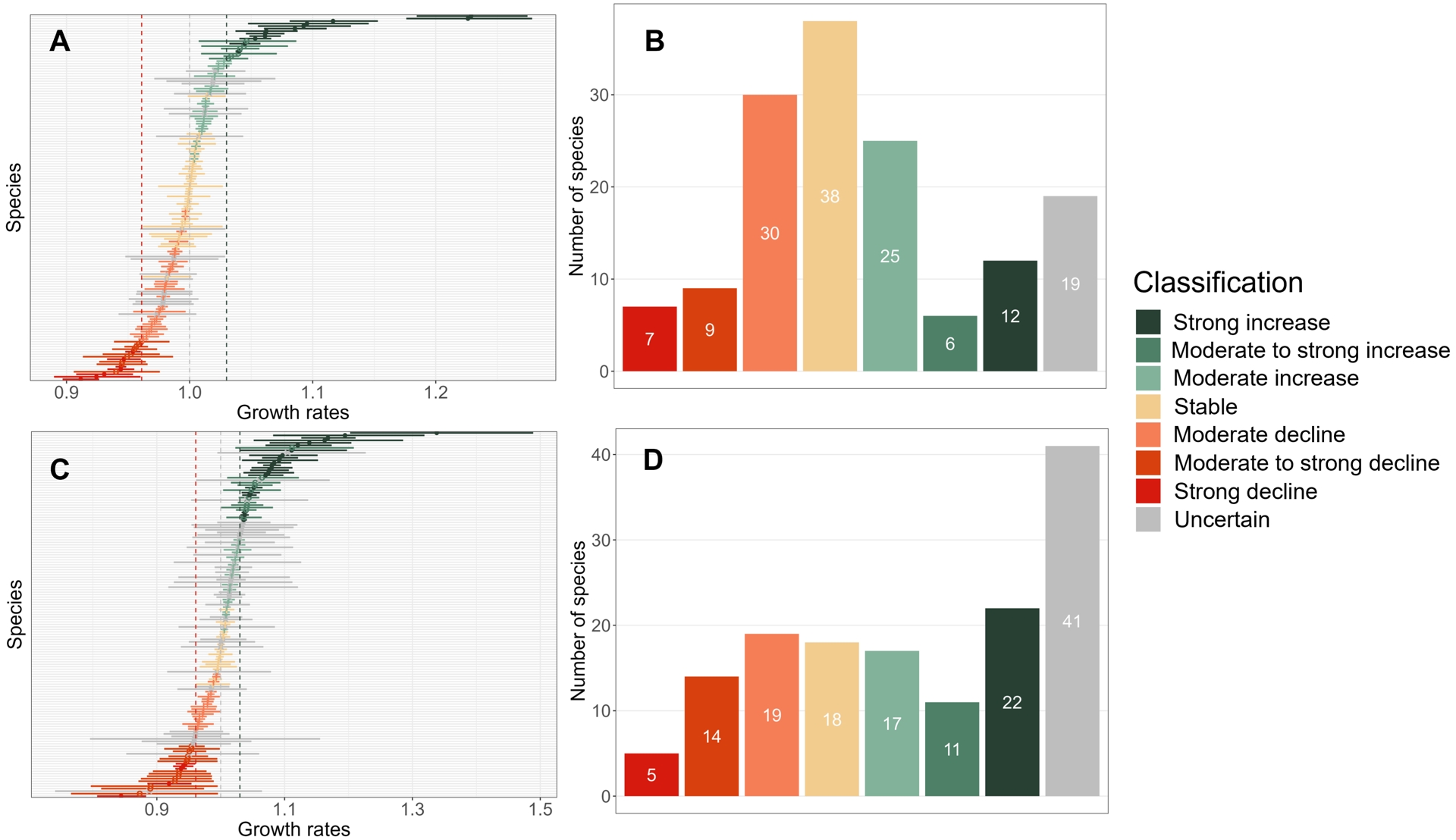
Over the shorter 2014–2023 period, model convergence was achieved for 145 out of 148 species. Trend estimates over the last ten years range from −0.169 (CI = [−0.215; −0.124]) for the Eurasian tree sparrow Passer montanus, corresponding to an annual growth rate of 0.844 (CI = [0.807; 0.883]), to 0.291 (CI = [0.184; 0.398]) for the western cattle egret Bubulcus ibis, i.e. an annual growth rate of 1.338 (CI = [1.20Z; 1.489]). These extremes represented respectively a decrease of 78.2% and an increase of 1274% over the ten-year monitoring period. Standard errors for these trend estimates are on average 0.0191, which is more than two times larger than for trend estimates over the 2001–2023 period (0.0079).
Patterns of trend classification are similar for the last ten years and for the 23-year period (Figure 2). A little more than a third of trends over the last ten years are classified as either “stable” (18 species) or “uncertain” (41 species), though we note an increase in the number of uncertain trends that is consistent with both the decrease in the available number of observations and the resulting increase in standard errors. As for the 23-year period, declining and increasing trends are evenly distributed (50 increasing species population trends against 38 declining). However, moderate trends tend to be less frequent, with 17 “moderately increasing” species population trends (resp. 19 “moderately decreasing” trends) compared to the 23-year period. Also, in the last ten years, there has been a reinforcement of species with a strong increase in abundance (from 12 to 22 species) and no such change regarding strong declines in abundance (from seven to five species). All species estimated trends and classifications over the 2014–2023 period are available in Appendix 2.
Estimating linear trends over a long period (2001–2023), however, masks more complex temporal patterns in abundance, which can be uncovered by comparing long (2001–2023) vs. shorter (2014–2023) term trends, or more finely by examining the non-linear patterns illustrated by the outputs of the GAMM (Appendix 6). Looking at the changes in trend classification between the 2001–2023 and the 2014–2023 periods for the 125 species for which models converged for both periods and for which trends were not “uncertain” in both periods (Figure 3), we found that species frequently changed trend classes across the two periods, sometimes with a change in the direction of the trend, or with a jump of one or more classes (e.g, from “moderate increase” to “strong increase”). These changes thus covered a variety of situations, from accelerated declines (e.g. the Wood warbler Phylloscopus sibilatrix) to recent recoveries, e.g. the Goldfinch Carduelis carduelis, or Cetti’s warbler Cettia cetti, for which the temporal trends in abundance produced by the GAMM are strongly non-linear (Figure 4). For Cetti’s warbler, examining the 2001–2023 linear trend thus says nothing of the initial decline between 2001 and 2012. Finally, some species show no change in trend classes between the two periods, as is the case with the long-term stability of the Carrion crow Corvus corone (Figure 4).
Alluvial plot showing the relationships between bird population trends over the 2001–2023 and the 2014–2023 periods. Each ribbon corresponds to a bird species. Five species for which a model did not converge for one of the periods and 18 species with uncertain trends for both periods (i.e., transitions from “Uncertain” to “Uncertain”) were not represented to improve readability.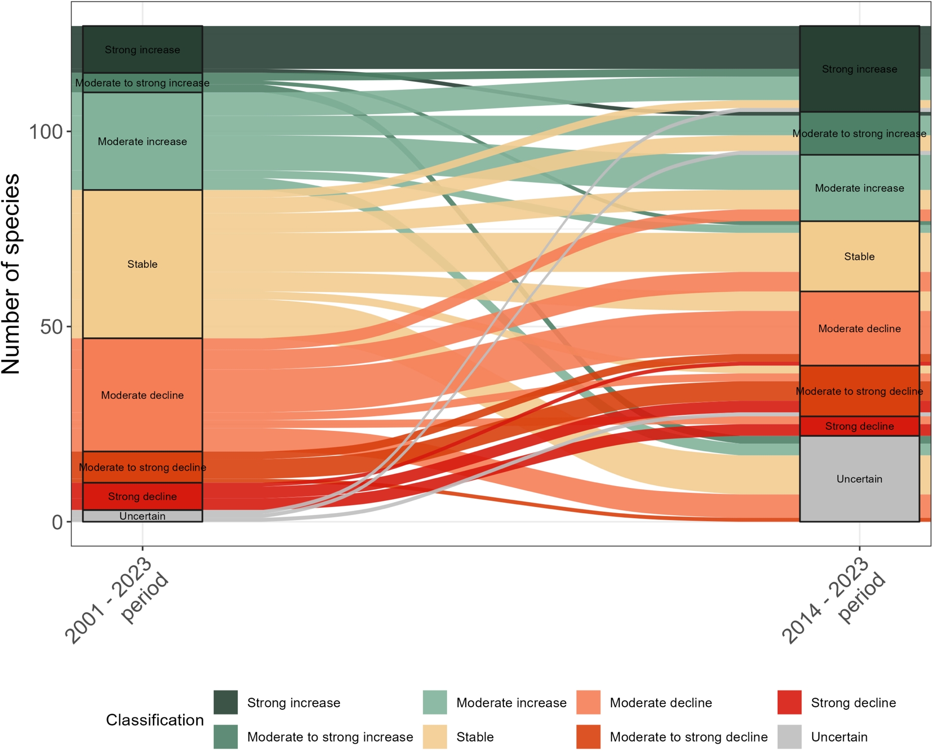
Examples of temporal trends in abundance for four bird species. The orange line corresponds to the temporal trend smoothed over the 2001–2023 period, with the orange ribbon representing uncertainty. Orange dots correspond to ratios of abundance between each year and the reference year. Blue and red lines correspond to uncertainty associated with the population trend estimated over the 2001–2023 period (resp. 2014–2023 period). Blue and red numbers on the left of the plot indicate the estimated annual growth rate for the 2001–2023 period (resp. 2014–2023 period). Stars on the right of the plot specify the significance of these estimates.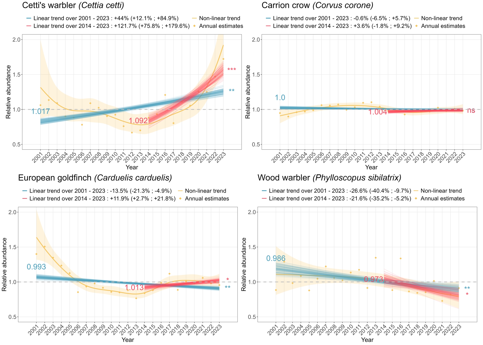
An absence of classification change in estimated population trends is not equivalent to an absence of absolute change in estimated population trends. For example, though the Eurasian golden oriole Oriolus oriolus population trend is classified as “moderately increasing” for both periods, the estimated annual growth rate increased from 1.005 to 1.029 (see Appendix 1 and 2), suggesting a recent stronger increase for this species. However, studying all changes in estimated trends between 2001–2023 and 2014–2023, we found that differences in estimates are centered around 0, with a slightly positive mean difference of 8.68 × 10⁻³ (CI = [3.33 × 10⁻³; 1.40 × 10⁻²]) corresponding to a mean ratio of 1.0087 (CI = [1.0033; 1.0141]).
Looking at population trends within groups of species habitat specialization, we notice that, for the 2001–2023 period, most habitat generalist species show “stable” (50%) or “moderately increasing” (21.4%) population trends, with no strong declines recorded. In contrast, forest specialists display a high proportion of populations with declining trends (50%), relatively few with stable trends (16.7%) but still a substantial proportion whose trends are increasing (33.3%). Urban specialists show a similar bimodal pattern, with 54% of species displaying declining trends, while 38.5% display increasing trends. The majority of farmland specialist species populations are declining (41.6%) or stable (37.5%) with relatively few increasing population trends (16.7% moderately increasing, and no strong increase).
These patterns slightly differ over the shorter 2014–2023 period (Table 4), with more numerous strongly increasing population trends among farmland specialist species, and a larger number of uncertain trends, particularly among “other” species.
When adding historical data collected from 1989 to 2001 with a different protocol (see methods) to estimate population trends over the period covering both protocols (1989–2023), model convergence was achieved for 107 species only (Appendix 3). The estimated trends in abundance are very similar to the ones obtained for the 2001–2023 period, with a mean difference of −2.02 × 10⁻⁴ (CI = [−7.94 × 10⁻⁴; 3.90 × 10⁻⁴]) and a maximum absolute difference of 1.51 × 10⁻². This is almost ten times less than the maximum difference observed between the 2001–2023 and the 2014–2023 periods (1.37 × 10⁻¹), suggesting that observations made before 2001 contribute only marginally to the 1989–2023 estimated trends, mainly due to their scarcity compared to the amount of data collected since 2001.
3.1.1. Plant species population trends
The estimation of plant population trends over the 2009–2023 period reached convergence for all 181 plant species. These trend estimates ranged from −0.106 (CI = [−0.197; −0.015]) for the common box Buxus sempervirens corresponding to a growth rate of 0.899 (CI = [0.821; 0.984]), to 0.100 (CI = [0.053; 0.147]) for the dandelion Taraxacum officinale corresponding to a growth rate of 1.105 (CI = [1.055; 1.158]). These extremes represented respectively a decrease of 77.4% and an increase of 307.7% over the 15-year monitoring period. Standard errors for these trend estimates were on average 0.0256, which is about three times larger than for bird species.
Most plant species trends over the 15-year period were classified as “uncertain” (126 species), i.e., the estimation was not precise enough to conclude for 70% of species. For the remaining species, we observed fewer increasing than declining population trends (respectively 15 and 32 species) as well as an over-representation of trends categorized as “moderately to strongly” increasing (9 species) or declining (23 species). All species estimated trends and classifications over the 2009–2023 period are available in Appendix 4.
Turning to the estimation of plant population trends over the last ten years, model convergence was achieved for all 178 species out of 181 (Figure 5). These trend estimates over the last ten years ranged from −0.209 (CI = [−0.300; −0.117]) for the tor-grass Brachypodium pinnatum corresponding to an annual growth rate of 0.811 (CI = [0.740; 0.889]), to 0.235 (CI = [0.139; 0.332]) for the dandelion Taraxacum officinale corresponding to an annual growth rate of 1.265 (CI = [1.149; 1.394]). These extremes represented respectively a decrease of 84.8% and an increase of 731.7% over the last ten-year monitoring period. Standard errors for these trend estimates were on average 0.0405, which is around 1.5 times larger than for trend estimates over the 2009–2023 period. All species estimated trends and classifications over the 2014–2023 period are available in Appendix 5.
Plant population trend estimates and classification for the 2009–2023 (A and B) and the 2014–2023 (C and D) periods. In panels A and C, error bars associated with plant population trend estimates represent 95% confidence intervals. Histograms on panels B and D indicate the number of plant species per class of population trend.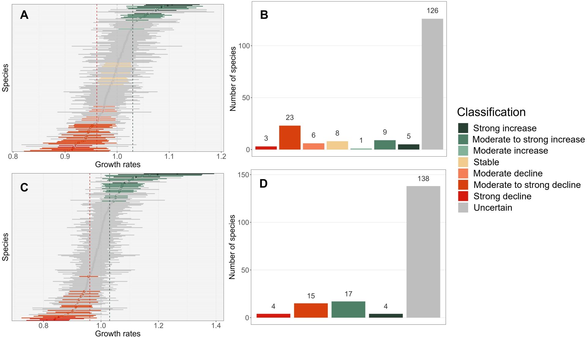
The pattern obtained in terms of trend classification for the last ten years did not differ much from the one obtained for the 15-year period, except that most species population trends categorized as “stable” over the 2009–2023 period switched to “uncertain” over the last ten-year period and that some species switched from an “uncertain” trend to a “moderate to strong increase” or “moderate to strong decline” trend (Figure 5). Yet, when comparing trend classification across the two time periods, the few changes in trend classes were diverse, as was the case for birds (Figure 6), including one accelerated increase (the English ryegrass Lolium perenne, Figure 7), long-term stability (e.g. blackberry, Rubus fruticosus, Figure 7) or transition to “uncertain” trends (e.g. The Traveller’s Joy Clematis vitalba, Figure 7). As for birds, the smoothed non-linear trends uncover finer temporal patterns (Appendix 7), such as the recent decline in a species population that appeared to be formerly stable over long- and short-term trends (Buxus sempervirens, Figure 7).
Alluvial plot showing the relationships between plant population trends over the 2009–2023 and the 2014–2023 periods. Each ribbon corresponds to a plant species. To improve readability, the 106 species with uncertain trends for both periods (i.e., transitions from “uncertain” to “uncertain”) were not represented.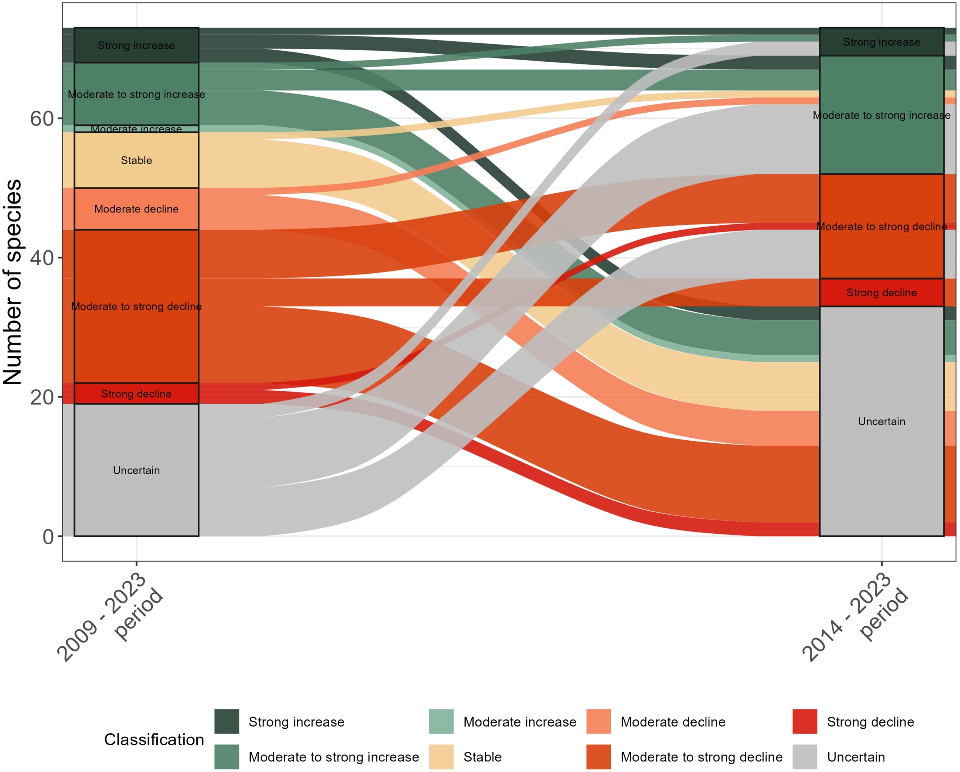
Examples of temporal trends in abundance for four plant species. The orange line corresponds to the temporal trend smoothed over the 2009–2023 period, with the orange ribbon representing uncertainty. Orange dots correspond to ratios of abundance between each year and the reference year. Blue and red lines correspond to uncertainty associated with the population trend estimated over the 2009–2023 period (resp. 2014–2023 period). Blue and red numbers on the left of the plot indicate the estimated annual growth rate for the 2009–2023 period (resp. 2014–2023 period). Stars on the right of the plot specify the significance of these estimates.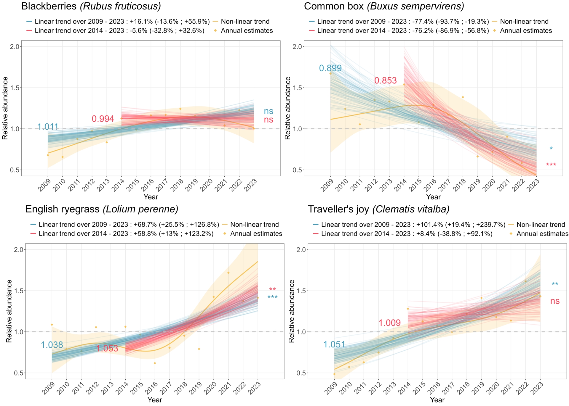
4. Discussion
In this paper, we present an analysis pipeline for estimating the population trends of multiple species across different taxa and time periods. This pipeline complements existing tools, in particular TRIM 3 (Pannekoek and Van Strien, 2005), by being more versatile for various data types, including occurrence data. We demonstrate this in our analysis of plant species. While we did not implement all TRIM 3 features, such as observation weighting, or missing data imputation, we leveraged mixed models and the glmmTMB package (Brooks et al., 2017), offering users flexibility in model parametrization. We also focused on result visualization and interpretation, proposing new graphical representations of population trends that include a trend over the entire period of the data, a trend over the last ten years, and a smoothed trend to capture non-linear or even non-monotonous patterns. These figures are automatically generated for each species if models converge. Drawing from the IUCN Red List framework (IUCN, 2012) and the PECBMS classification, we developed a seven-class categorization that is better suited for temporal trend analysis. Our classification is more sensitive to uncertainty and reduces the risk of biologically irrelevant abrupt category changes. Finally, for transparency, we saved all raw models and main results in tables, so that users can access them beyond visual representations.
4.1. Overview of population trends in birds and plants
The analysis pipeline that we propose uses data from citizen science monitoring schemes targeting bird and plant species, and provides an unprecedented overview of the current dynamics of common biodiversity in France. While annual bird population trends were already produced from the same dataset using TRIM 3 (Fontaine et al., 2020), this is the first time that plant population trends have been made available. Looking at the population trends over the entire monitoring periods (2001–2023 for birds and 2009–2023 for plants), we found almost as many bird species with declining populations as those with increasing ones, and slightly more plant species with declining populations than with increasing ones. For bird species, these results may appear to contrast with recent studies highlighting bird abundance decline in Europe or France (Lehikoinen et al., 2019; Rigal, Dakos, et al., 2023). Such studies usually tend to focus on smaller sets of bird species consisting of habitat specialists (e.g. farmland, woodland, or mountain species), for which it is worth noting that we also found a majority of declining trends (Tables 3 and 4). In contrast, our analysis covers all common bird species in France, including habitat generalists and exotic species with population sizes that are known to be mostly stable or increasing (Le Viol et al., 2012), similarly to what we found. Such a pattern of habitat generalist species showing increasing populations while habitat specialist species show declining ones is consistent with biotic homogenization (Devictor et al., 2008). However, our results further show that habitat specialization alone does not explain the variations in bird population trends. Indeed, although we found that 11 out of 14 habitat generalist bird species had stable or increasing populations, the remaining three species showed declining abundances (Dunnock Prunella modularis, Green woodpecker Picus viridis and Common cuckoo Cuculus canorus; see Appendix 1 and Supplementary material “Habitat Specialization”). Similarly, among habitat specialist species, 29 show decreasing trends (e.g. Meadow pipit Anthus pratensis or Tree sparrow Passer montanus), but 17 population trends are classified as increasing (e.g. Jackdaw Corvus monedula or Hawfinch Coccothraustes coccothraustes) and 14 as stable (e.g. Hoopoe Upupa epops or Kestrel Falco tinnunculus). These results therefore suggest that we need to go beyond habitat specialization to fully understand bird population trends. We should consider other potential response traits, such as trophic specialization (Bowler et al., 2019).
An important caveat when interpreting temporal trends is that they might be sensitive to changes in species detectability that are associated with their life cycles. Thus, a change in phenology, which has already been highlighted for birds (Romano et al., 2023) and for plants (Piao et al., 2019), could lead to the detection of a temporal trend in detectability, instead of an actual temporal change in abundance or occurrence. To be precise, because the STOC protocol encourages recording sessions to occur around the same dates every year, a slight phenological advance or delay could lead to the detection of an increasing (resp. decreasing) trend in abundance. Yet, the potential impact of phenological changes on the resulting estimated trends could be tested by incorporating the exact recording session dates into the analysis, so as to model phenology in addition to trends in abundance. Currently, this is done for plants, although phenology might be better estimated using at least a quadratic effect on the observation date. Others have done so, such as (Schmucki et al., 2016) for butterflies or (Moussus et al., 2009) for birds.
Turning to plants, the scarcity of studies on this topic in France makes it difficult to compare our results to previous work (but see (Fried et al., 2009) for arable weeds). Nonetheless, our results are consistent with patterns observed in other countries, such as more numerous losses than gains in frequency for plants in Germany (Jandt et al., 2022). Overall, we observed that many bird and plant species exhibited either declining or increasing population trends. This indicates that the composition of common bird and plant assemblages is strongly changing, a result confirming previous studies, such as (Rigal, Devictor, Gaüzère, et al., 2022) for birds and (Bühler and Roth, 2011) for plants. While several studies have documented such changes in French bird communities (e.g. Devictor et al., 2008; Lorel et al., 2021), the consequences for the composition of plant communities in France remain to be examined.
4.2. Non-linearity in population dynamics
Our analysis pipeline, by estimating linear population trends over multiple time periods, showed that trends are highly dependent on temporal depths. Indeed both the direction and speed of species’ growth rates vary depending on the considered time-period. This is consistent with recent studies that point out the non-linearity of temporal trends in population abundance or occurrence, as well as the impact of the chosen time period on these estimated trends (Duchenne et al., 2022). Such non-linearities in population trends call for detailed and species-specific interpretations. For instance, the population trend of Cetti’s warbler Cettia cetti goes from “moderate increase” in 2001–2023 to “strong increase” during the 2014–2023 period. This sedentary and insectivorous species is highly vulnerable to harsh winters. It has experienced important population collapses in the past after the 1984–1985 and 1986–1987 cold winters in France (Issa and Muller, 2015). It is likely that this species has benefited from global warming and mild winters in recent years, such that its range is shifting northward in Western Europe (Clement, 2020). However, the explanation for the differences in trends observed over longer vs. shorter time periods is not always straightforward: the changing trends of the Wood warbler Phylloscopus sibilatrix may be attributable to a combination of factors, including changing forest management, locally or on their wintering grounds, prey availability, and climate change; however, the exact contribution of each potential driver remains uncertain and needs to be investigated. These examples all illustrate the interest of highlighting trends in different timeframes to get a finer insight into bird population dynamics.
We are aware that our current methodology, which consists of splitting the timeline to cover either the whole monitoring period or the last ten years, cannot perfectly encompass the dynamics of species populations. As a first step, we chose to illustrate this non-linearity using generalized additive models to calculate smoothed trends over the entire period. One major interest of this trend representation is to reveal complex population dynamics that cannot be properly described using linear trends, even when considering different time periods. For instance, the European hoopoe Upupa epops is considered as “stable” with our categorization during both time periods. However, its annual variations (Appendix 6, pp. 2) show remarkable cyclical dynamics, with a period of seven years. This pattern could be related to the population dynamics of one of its important prey (Barbaro and Battisti, 2011), the pine processionary moth Thaumetopoea pityocampa, whose population outbreaks every seven to nine years in France (Li et al., 2015). However, smoothing trends were only implemented as a visual tool in the pipeline, and further development is needed to properly characterize and quantify this non-linearity . (Rigal, Devictor and Dakos, 2020) for example, suggest the use of a 2nd order polynomial regression, which allows for non-linearity of the time effect, while still being understandable and biologically relevant.
4.3. Challenges and limitations in trend estimation
With this non-linearity in mind, and given that pressures on biodiversity have started long before the starting dates of biodiversity monitoring schemes (Mihoub et al., 2017), one of our objectives was to challenge our current 2001 baseline and study what would happen if we went back further in time regarding bird population trends. Our results, however, were impacted by the low number of observations available before 2001, which caused trends to be mostly driven by observations made after 2001. This finding was illustrated by the small number of differences observed between estimated trends over the 1989–2023 period and the 2001–2023 period. Such limitations related to data availability are also highlighted by the higher uncertainty associated with trends over the last ten years for both bird and plant species. Similarly, the impact of sampling effort was illustrated by the overall wider confidence intervals observed for plant population trends compared to those observed for birds, as well as the high number of plant species with population trends classified as “uncertain”. This is at least partly due to the fact that the plant monitoring scheme is more recent than the bird one and relies on fewer monitored squares. These results emphasize the difficulty of detecting very short-term changes in population dynamics, and the need to be thoughtful when defining both the sampling effort and focus period, as stated in (Rigal, Devictor and Dakos, 2020; Duchenne et al., 2022). It also suggests that more work need to be done to understand how each observation contributes to trend estimation and to deal with any imbalance in sampling efforts across monitoring schemes and over time. One possible solution could be to weight observations so that each year contributes equally to the trend, which is the principle behind the data imputation method offered by the tool TRIM 3 (Pannekoek and Van Strien, 2005). This idea of weighting observations depending on a representativity criterion has also been implemented in well-known indicators such as the Living Planet Index (Westveeret al., 2022).
Another limitation comes from the data themselves. When trying to routinely analyze multiple species, we aimed at combining both generic and relevant model specifications. This was made difficult by the nature of the collected data, which consists of counts of multiple individuals at the same time, leading volunteers to round off their observations to the nearest ten. This is particularly true for the bird dataset with abundance distributions showing a higher frequency of tens, thus questioning the choice of the underlying distribution law. To further assess model adequacy with respect to data structure and goodness-of-fit, we conducted diagnostic tests using the DHARMa package (Hartig, 2024). We did not detect overdispersion issues for either plant or bird models, indicating a good fit and the ability to handle large variance with the chosen beta-binomial and negative binomial distributions, for plants and birds, respectively. However, we did find underdispersion in 88 out of 181 plant species, and in approximately one third of the bird species (56 out of 148). Notably, the strongest underdispersion occurred in gregarious birds. This is likely due to a stronger rounding bias in observations (as discussed above), which may have resulted in lower variances than expected. While underdispersion leads to fewer concerns than overdispersion, as it tends to produce more conservative estimates (Bolker, 2024), it still warrants consideration: plant trends are notably affected by relatively large confidence intervals. Therefore, new functionalities and data treatments should be explored to address this issue. One solution may be to use distributions that specifically deal with both underdispersion and overdispersion, such as the Conway–Maxwell–Poisson distribution or the generalized Poisson distribution for count data, and the quasi-binomial for occurrence data. For birds, an additional step in data processing could also be considered to correct rounding biases, such as adding random noise to counts.
4.4. Applications and next steps for the pipeline
The proposed pipeline is a valuable tool for systematically documenting temporal changes in the abundance of common birds or plants. It provides a proof-of-concept that can be readily adapted to other monitoring schemes targeting diverse taxa, for which no systematic appraisal of temporal trends may exist. In France, citizen science monitoring schemes exist for bats (Vigie-Chiro) and butterflies (STERF), which are two obvious candidates for such an extension. Nevertheless, several areas for improvement have been identified. First, although the pipeline can already handle different measures/proxies of abundance, namely count and frequency data, it does not cover biomass data, which may be frequent in insect monitoring (see Hallmann et al., 2017) or percent-cover data, which is common in plant monitoring. The handling of such data can, however, be easily implemented in the pipeline, as it requires standard linear mixed models with a Gaussian distribution. Second, the thresholds used to classify species into categories of temporal trends, from strong decline to strong increase, were directly inspired by the IUCN categories, but may need to be tailored to the specificities of each taxonomic group. Indeed, IUCN categories may be operational for groups for which count data are easily collected (large animals such as birds and mammals), but they may be less relevant for other groups with different abundance measurements and fewer data, such as plants. This would reduce the number of species in the “uncertain” category and provide a better vision of the current dynamics of biodiversity across multiple taxonomic groups. Finally, to make the graphical outputs of the pipeline accessible to a wide audience, a solution could be to exploit R functionalities, such as the RShiny package (Chang et al., 2025), which is especially adapted to online sharing with an interactive user interface. By connecting our routine to a web application, users could update graphics depending on the selection of species, temporal frames or even relevant thresholds.
Acknowledgements
We wish to thank all the volunteers who collected data for the STOC and Vigie-flore schemes, without whom these analyses and insights on bird and plant population dynamics would not have been possible. We also thank Luc Barbaro for his hypotheses on the population dynamics of the Eurasian hoopoe.
Declaration of interests
The authors do not work for, advise, own shares in, or receive funds from any organization that would benefit from this article, and have declared no affiliation other than their research organizations.