

1 Introduction
The phenomenon of thermally induced spin crossover (SCO) between the low-spin (LS) and high-spin (HS) states of transition metal complexes has been thoroughly studied by different experimental techniques [1]. Recently, computational studies based on the density functional theory (DFT) methodology were also carried out on some SCO complexes [2–11]. These calculations aimed to determine the energy difference between the HS and LS states, as well as to calculate the vibrational frequencies.
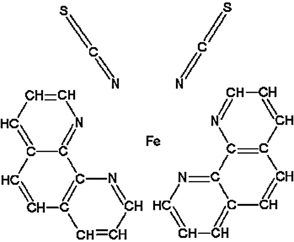
The molecular vibrations play an important role in the SCO phenomenon since the HS form is stabilized at high temperatures by its higher entropy of mostly vibrational origin [12,13]. Calculation of molecular vibrations is thus crucial for the study of the SCO mechanism. However, it is not obvious to estimate the reliability of frequency calculations, because (i) the measured vibrational spectra are always incomplete due to selection rules and intensity reasons and (ii) they do not provide the assignment of vibrational modes. In fact, a reliable assignment of experimental spectra is possible only on isotope labeled compounds. Therefore, we decided to focus on the Fe(phen)2(NCS)2 complex (Fig. 1) for which the most extensive experimental data are available including 54Fe–57Fe and 14N–15N isotope labeling [13,14]. Moreover, computational results have also been published employing the DFT methodology with BP86 functional: Baranovic and Babic [7] used the 6-311G(d) basis set and Brehm et al. [8] the TZVP basis set. In Ref. [7], 54Fe–57Fe frequency shifts were reported as well. In the present paper we calculate vibrational spectra with 54Fe–57Fe and 14N–15N isotope substitutions employing the B3LYP method and compare our results to experimental as well as calculated (BP86) literature data. These two functionals have—in general—been considered the most suitable for the evaluation of vibrational spectra of transition metal complexes [16].
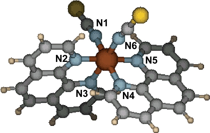
Geometry of the LS isomer of Fe(Phen)2(NCS)2 calculated with B3LYP/6-31G(d).
2 Computational methods
DFT calculations were performed with the Gaussian 98 program package [17]. The B3LYP functional was used with two different basis sets: 3-21G and 6-31G(d). X-ray diffraction data [18] were used initially in the structure optimization, which were carried out first with the 3-21G and consequently with the 6-31G(d) basis set using the Berny optimization algorithm [19]. The structures were fully optimized without any constraints. After completion of the optimization, vibrational frequencies were calculated with both basis sets within the harmonic approximation.
3 Results and discussion
3.1 Structural analysis
In both spin states and with both computational methods we obtained the expected C2 symmetry for the molecule. Tables 1a and 1b show a selection of bond distances and angles to compare the experimental and calculated structures in the LS and HS states (see also Fig. 2). On the whole, we found that the B3LYP functional with 6-31G(d) basis set performs in prediction of structural changes with a comparable precision than the BP86 [7,8] method. The values of bond angles and lengths not involving the Fe atom are reproduced with good accuracy. The deviations from the experimental data were found somewhat larger in the HS state. On the other hand, more important differences were found in structural parameters involving the central metal atom. The general tendency—increase of Fe–N bond distances when going from the LS to HS state—was well reproduced, though in the LS case the calculations underestimate somewhat these bond lengths. In the HS state this was observed only for the Fe-NCS (Fe–N1, Fe–N6) distances, the others are overestimated. It is interesting to note that in the LS state the larger basis set leads to smaller errors, in contrast with the HS state situation. In this latter case, the calculation with 6-31G(d) basis well overestimates the Fe–N3 and Fe–N4 distances. The methods used by Baranovic and Babic [7] could not reproduce the correct order for the Fe–N2 and Fe–N3 distances. Therefore it is interesting to see that the B3LYP functional with the relatively small 3-21G basis set was able to do it (presumably by chance), while with the bigger 6-31G(d) not.
Experimental [18] and calculated Fe–N distances (Å) in the Fe(Phen)2(NCS)2 SCO complex
| LS state | |||
| X-ray (130 K) | B3LYP/3-21G | B3LYP/6-31G(d) | |
| Fe–N1 | 1.958 (4) | 1.896 | 1.934 |
| Fe–N2 | 2.014 (4) | 1.934 | 1.985 |
| Fe–N3 | 2.005 (4) | 1.926 | 1.994 |
| Fe–N4 | 2.005 (4) | 1.926 | 1.994 |
| Fe–N5 | 2.014 (4) | 1.934 | 1.985 |
| Fe–N6 | 1.958 (4) | 1.896 | 1.934 |
| HS state | |||
| X-ray (295 K) | B3LYP/3-21G | B3LYP/6-31G(d) | |
| Fe–N1 | 2.057 (4) | 1.994 | 2.010 |
| Fe–N2 | 2.198 (3) | 2.222 | 2.214 |
| Fe–N3 | 2.212 (3) | 2.243 | 2.320 |
| Fe–N4 | 2.212 (3) | 2.243 | 2.320 |
| Fe–N5 | 2.198 (3) | 2.222 | 2.214 |
| Fe–N6 | 2.057 (4) | 1.994 | 2.010 |
Selected experimental [18] and calculated bond distances (Å) and bond angles (°) in the Fe(Phen)2(NCS)2 SCO complex
| LS state | HS state | |||
| X-ray (130 K) | B3LYP/6-31G(d) | X-ray (295 K) | B3LYP/6-31G(d) | |
| C2b–N2 | 1.355 | 1.362 | 1.366 | 1.358 |
| C2a–N2 | 1.335 | 1.333 | 1.337 | 1.331 |
| C3b–N3 | 1.361 | 1.364 | 1.373 | 1.356 |
| C3a–N3 | 1.331 | 1.333 | 1.327 | 1.327 |
| C2b–C3b | 1.429 | 1.428 | 1.421 | 1.442 |
| C1–N1 | 1.140 | 1.183 | 1.158 | 1.188 |
| S1–C1 | 1.632 | 1.634 | 1.628 | 1.626 |
| N2–Fe–N3 | 81.8 | 82.3 | 76.1 | 73.1 |
| N1–Fe–N3 | 95.3 | 87.4 | 103.2 | 97.5 |
| N1–Fe–N2 | 89.1 | 88.9 | 89.6 | 86.5 |
| C3b–N3–Fe | 112.5 | 112.6 | 114.3 | 117.1 |
| C3a–N3–Fe | 129.5 | 129.9 | 126.7 | 123.5 |
| C3a–Fe–C3b | 117.8 | 117.5 | 118.9 | 118.6 |
| C2b–N2–Fe | 113.1 | 113.1 | 113.0 | 113.6 |
| C2a–N2–Fe | 129.5 | 128.5 | 128.4 | 127.4 |
| C2a–N2–C2b | 117.4 | 118.1 | 118.6 | 118.4 |
| C1–N1–Fe | 165.6 | 168.4 | 167.0 | 169.3 |
| C2b–C3b–N3 | 116.6 | 116.0 | 117.7 | 117.6 |
| C30–C3b–N3 | 123.6 | 123.8 | 121.8 | 122.7 |
| C3b–C2b–N2 | 115.9 | 115.8 | 118.9 | 117.6 |
| C20–C2b–N2 | 123.7 | 123.7 | 121.3 | 122.8 |
| S1–C1–N1 | 179.5 | 178.9 | 179.4 | 179.1 |
Atom numbering for the Fe(Phen)2(NCS)2 complex.
3.2 Vibrational spectra
The Fe(phen)2(NCS)2 molecule consists of 51 atoms and therefore 147 fundamental vibrational modes are expected. Among these we found 49 below 600 cm–1, 82 between 600 and 2200 cm–1, and 16 above 3100 cm–1 in both spin states. Brehm et al. [8] have found 51 modes below 600 cm–1 and 80 between 600 and 2200 cm–1 in both spin states. Baranovic and Babic [7] calculated 49 modes below 600 cm–1 in the LS state and 48 in the HS state. As mainly the vibrations below 600 cm–1 are expected to contribute to the entropy change which accompanies the SCO [13,20], we will confine the following analysis to this frequency range.
Tables 2a and 2b exhibit the calculated Fe displacements and the frequency shifts upon 54Fe–57Fe and 14N–15N isotope substitutions. For comparison we included the experimental IR spectra published by Takemoto and Hutchinson [14] and Hoefer [15] including 54Fe–57Fe and 14N–15N isotope substitutions, respectively. We have highlighted with bold letters the experimental data with a measured isotope shift larger than 1 cm–1 (taking into account the experimental precision). In the case of calculated isotope shifts, we fixed this limit at 0.5 cm–1. Experimental frequencies displaying significant isotope shifts are also given in Tables 3a and 3b together with frequencies calculated using the BP86 [7,8] and B3LYP functionals.
Comparison of calculated frequencies (cm–1) and frequency shifts (cm–1) upon 54Fe–57Fe and 14N–15N isotope substitutions (LS state)
| Calculated frequencies (54Fe) | Calculated frequency shifts (54/57Fe) | Experimental frequencies a | Experimental frequency shifts | Calculated frequency shifts (14/15N) | Experimental frequencies b | |
| 1 | 14.7 | 0.0 | 0.0 | |||
| 2 | 16.8 | 0.0 | 0.0 | |||
| 3 | 20.5 | 0.0 | 0.0 | |||
| 4 | 20.6 | 0.0 | 0.0 | |||
| 5 | 28.0 | 0.0 | 0.0 | |||
| 6 | 37.6 | –0.1 | –0.1 | |||
| 7 | 40.9 | 0.0 | 0.0 | |||
| 8 | 79.6 | 0.0 | –0.2 | |||
| 9 | 84.0 | –0.1 | 107.0 | – | 0.0 | 106.0 |
| 10 | 123.9 | 0.0 | 117.0 | – | –1.3 | |
| 11 | 154.9 | –0.1 | 132.0 | 0.0 | –0.4 | 134.0 |
| 12 | 167.9 | 0.0 | 164.0 | 0.0 | –0.4 | 163.0 |
| 13 | 175.1 | 0.0 | –0.3 | |||
| 14 | 177.1 | –0.1 | 187.0 | 0.0 | –0.4 | 185.0 |
| 15 | 182.3 | 0.0 | 192.5 | –0.5 | –0.3 | 192.0 |
| 16 | 203.1 | 0.0 | –2.1 | |||
| 17 | 210.8 | –0.1 | 212.5 | 0.0 | –3.2 | 212.0 |
| 18 | 218.8 | –0.1 | 235.0 | 0.0 | –4.2 | 235.0 |
| 19 | 231.9 | 0.0 | –0.3 | |||
| 20 | 235.2 | 0.0 | –0.3 | |||
| 21 | 247.4 | –0.1 | 243.0 | 0.0 | –2.5 | 244.0 |
| 22 | 247.9 | 0.0 | –2.4 | 251.0 | ||
| 23 | 291.4 | –0.2 | 286.0 | 0.0 | –0.4 | 286.0 |
| 24 | 295.9 | –1.0 | 298.5 | –0.8 | –0.1 | 297.0 |
| 25 | 295.9 | 0.0 | –0.1 | |||
| 26 | 308.4 | –0.3 | 311.0 | – | –0.2 | |
| 27 | 372.8 | –6.7 | 371.0 | –6.0 | –0.3 | 366.0 |
| 28 | 384.3 | –5.3 | 379.0 | –5.0 | –0.4 | 375.0 |
| 29 | 384.5 | –5.4 | 379.0 | –5.0 | –0.2 | 375.0 |
| 30 | 437.2 | –0.1 | 0.0 | 421.0 | ||
| 31 | 440.2 | –0.9 | 429.5 | –0.5 | 0.0 | 428.0 |
| 32 | 441.2 | –0.1 | 436.0 | – | –0.1 | 434.0 |
| 33 | 448.3 | –0.1 | 455.1 | –0.3 | –0.1 | |
| 34 | 467.6 | –0.2 | 475.7 | –3.2 | 475.0 | |
| 35 | 470.8 | 0.0 | 475.7 | 0.0 | –3.6 | 475.0 |
| 36 | 471.2 | –0.2 | 475.7 | –3.4 | 475.0 | |
| 37 | 478.4 | –0.5 | 480.2 | –3.7 | 479.0 | |
| 38 | 480.2 | –0.2 | 480.2 | –0.3 | –2.4 | 479.0 |
| 39 | 481.9 | –0.4 | 480.2 | –1.8 | 479.0 | |
| 40 | 501.7 | –0.2 | –0.3 | 486.0 | ||
| 41 | 507.0 | –0.4 | 504.4 | 0.0 | –0.5 | 503.0 |
| 42 | 517.9 | 0.0 | 513.3 | –0.2 | 0.0 | |
| 43 | 518.0 | 0.0 | 0.0 | |||
| 44 | 542.4 | –0.9 | 528.5 | –1.7 | –0.3 | 528.0 |
| 45 | 546.0 | –0.9 | 532.6 | –1.6 | –0.1 | 531.0 |
| 46 | 556.7 | 0.0 | 0.0 | |||
| 47 | 558.4 | 0.0 | 560.0 | 0.0 | ||
| 48 | 569.7 | 0.0 | 0.0 | |||
| 49 | 570.5 | 0.0 | 0.0 |
a 100 K, 54Fe from Ref. [14], bold values refer to 54Fe–57Fe isotope shift greater than 1 cm–1.
b 25 K, 14N from Ref. [15], bold values refer to 14N–15N isotope shift greater than 1 cm–1 (the experimental frequency shifts for 14N–15N isotope exchange were not published).
Comparison of calculated frequencies (cm–1) and frequency shifts (cm–1) upon 54Fe–57Fe and 14N–15N isotope substitutions (HS state)
| Calculated frequencies (54Fe) | Calculated frequency shifts (54/57Fe) | Experimental frequencies a | Experimental frequency shifts | Calculated frequency shifts (14/15N) | Experimental frequencies b | |
| 1 | 11.4 | 0.0 | 0.0 | |||
| 2 | 11.9 | 0.0 | 0.0 | |||
| 3 | 14.6 | 0.0 | 0.0 | |||
| 4 | 15.4 | 0.0 | 0.0 | |||
| 5 | 20.9 | 0.0 | 0.0 | |||
| 6 | 22.8 | 0.0 | 0.0 | |||
| 7 | 25.9 | 0.0 | 0.0 | |||
| 8 | 60.7 | 0.0 | –0.3 | |||
| 9 | 77.0 | –0.1 | –0.1 | |||
| 10 | 89.1 | –0.1 | –0.4 | |||
| 11 | 92.4 | 0.0 | –0.4 | |||
| 12 | 105.7 | –0.1 | –0.7 | 109 | ||
| 13 | 116.0 | –0.3 | 126.0 | 0.0 | –0.7 | |
| 14 | 138.8 | –0.2 | –1.9 | 133 | ||
| 15 | 141.9 | –0.3 | –0.1 | |||
| 16 | 145.1 | –0.2 | –2.0 | |||
| 17 | 154.7 | –0.2 | 156.0 | 0.0 | –1.4 | 160 |
| 18 | 156.2 | –0.2 | 156.0 | 0.0 | –2.5 | 160 |
| 19 | 163.5 | –0.9 | 166.0 | – | –1.2 | 170 |
| 20 | 171.0 | –0.4 | 178.5 | 0.5 | –0.7 | |
| 21 | 202.9 | –3.1 | 220.0 | –4.5 | –1.0 | 226 |
| 22 | 237.1 | 0.0 | 0.0 | 222 | ||
| 23 | 238.6 | 0.0 | 235.0 | – | 0.0 | |
| 24 | 257.2 | 0.0 | 0.0 | |||
| 25 | 259.0 | –1.7 | 252.9 | –4.0 | –0.8 | 254 |
| 26 | 264.8 | –0.9 | 252.9 | –4.0 | –0.5 | 254 |
| 27 | 275.1 | –2.4 | 252.9 | –4.0 | –0.6 | 254 |
| 28 | 281.2 | –0.6 | 252.9 | –4.0 | –0.1 | 254 |
| 29 | 292.7 | –2.2 | 284.5 | 0.0 | –0.1 | 287 |
| 30 | 417.1 | 0.0 | 0.0 | |||
| 31 | 421.7 | 0.0 | 419.5 | 0.0 | 0.0 | 420 |
| 32 | 422.5 | 0.0 | 0.0 | |||
| 33 | 425.0 | 0.0 | 430.5 | 0.5 | 0.0 | 430 |
| 34 | 450.6 | 0.0 | 0.0 | |||
| 35 | 453.5 | 0.0 | 0.0 | |||
| 36 | 477.6 | 0.0 | 473.5 | 0.2 | –3.4 | 474 |
| 37 | 479.0 | 0.0 | 473.5 | 0.2 | –3.5 | |
| 38 | 483.3 | 0.0 | –1.9 | |||
| 39 | 483.5 | 0.0 | –0.3 | |||
| 40 | 488.5 | 0.0 | 485.0 | 0.5 | –3.6 | 487 |
| 41 | 489.0 | 0.0 | 485.0 | 0.5 | –2.4 | |
| 42 | 513.8 | 0.0 | 498.5 | 0.0 | –0.1 | |
| 43 | 514.8 | 0.0 | 512.5 | 0.5 | 0.0 | 513 |
| 44 | 517.8 | 0.0 | 0.0 | |||
| 45 | 518.1 | 0.0 | 0.0 | |||
| 46 | 556.7 | 0.0 | 0.0 | |||
| 47 | 557.4 | 0.0 | 0.0 | |||
| 48 | 563.4 | 0.0 | 0.0 | |||
| 49 | 565.4 | 0.0 | 0.0 |
a 298 K, 54Fe from Ref. [14], bold values refer to 54Fe–57Fe isotope shift greater than 1 cm–1.
b 25 K (LIESST), 14N from Ref. [15], bold values refer to 14N–15N isotope shift greater than 1 cm–1 (the experimental frequency shifts for 14N–15N isotope exchange were not published).
Comparison of measured and calculated frequencies (in cm–1) in the LS state. 54Fe–57Fe isotope shifts are given in parentheses.
| Measured frequencies (54Fe) [14] | Calculated frequencies [9] (56Fe) | Calculated frequencies [8] (54Fe) | Calculated frequencies [this work] (54Fe) |
| 298.5 (–0.8) | 291 | 293.3 (–1.3) | 295.9 (–1.0) |
| 371.0 (–0.6) | 375 | 372.1 (–5.9) | 372.8 (–6.7) |
| 379.0 (–0.5) | 377 | 379.4 (–4.8) | 384.3 (–5.3) |
| 429.5 (–0.5) | 432 | 434.7 (–1.4) | 440.2 (–0.9) |
| 528.5 (–1.7) | 526 | 529.9 (–1.3) | 542.4 (–0.9) |
| 532.6 (–1.6) | 556 | 536.4 (–1.4) | 546.0 (–0.9) |
Comparison of measured and calculated frequencies (in cm–1) in the HS state (bold values refer to 54Fe–57Fe isotope shift greater than 1 cm–1)
| Measured frequencies (54Fe) [14] | Measured frequency shifts [14] | Calculated frequencies [9] (56Fe) | Calculated frequencies [8] | Calculated frequencies [this work] |
| 166.0 | 0.0 | 163 | 160.6 | 163.5 |
| 220.0 | 4.5 | 198 | 196.3 | 202.9 |
| 252.9 | 4.0 | 282 | 265.7, 274.9, 282.5 | 259.0, 264.8, 275.1, 281.2 |
| 284.1 | 0.0 | 288 | 291.9 | 292.7 |
Four significant Fe isotope shifts are clearly discernible in the measured LS spectrum (at 371.0, 379.0, 528.5 and 532.6 cm–1). Each calculation method finds the two lower frequency modes with a relatively small error (< 5 cm–1). (In fact, both Baranovic and we find three peaks, but two of them are very close and are probably unresolved in the experimental spectra.) There is also a remarkably good agreement between the measured and calculated frequency shifts (5–6 cm–1). The same can be said for the two higher frequency modes as well, though in our case there is a somewhat larger difference between the calculated and measured frequencies. On the other hand, the magnitude of the isotope shifts is close to 1 cm–1 in each spectrum. It should be noted that Baranovic et al. found two more modes at 293.3 and 434.7 cm–1 being sensitive to the iron isotope substitution. For these we can correspond two measured peaks at 298.5 and 429.5, which have showed small measured shifts of 0.8 and 0.5 cm–1, respectively. In our calculations, we can also identify these peaks at 295.9 and 440.2 cm–1 displaying comparable isotope shifts. Let us finally note that, though they have not performed isotope substitution calculations, the frequencies computed by Brehm et al. can be straightforwardly correlated with our data (Tables 3a and 3b).
In the measured HS spectrum only two peaks at 220.0 and 252.9 cm–1 displayed Fe isotope shifts. According to our calculation there are seven vibrational modes with considerable isotope shift in the HS state. Taking into account the magnitude of the isotope shift, it is likely that the mode at 202.9 cm–1 corresponds to the measured peak at 220.0 cm–1. The four modes between 259.0 and 281.2 cm–1 correspond probably to the measured peak at 252.0 cm–1, which is very broad with a half width of approximately 30 cm–1. Concerning the calculated peak at 292.7 cm–1, there is a corresponding measured one, though without any measured isotope effect. However, this peak does not appear in the LS spectrum, which point to Fe–N stretching contribution in this vibration. Therefore, there might be a yet unrecognized isotope shift. The same can be said for the 163.5 cm–1 calculated peak. It is important to note, however, that all the seven calculated peaks with significant isotope shift were found by Baranovic et al. as well.
Hoefer has measured the frequency shifts upon 14N–15N isotope substitution in the NCS– ligand [15]. As there is no other published computed frequency shift for 14N–15N isotope substitution we cannot make the comparison between the computed data. In the LS state there are six peaks with measured shift more than 1 cm–1 on 14N–15N substitution and we found 12 calculated ones. However, several calculated frequencies are very close to each other; therefore nine calculated modes (210.8; 218.8; 247.4; 467.6, 470.8, 471.2; and 478.4, 480.2, 481.9 cm–1) could be connected to five measured peaks displaying shifts. There is one measured frequency (375.0 cm–1), for which the corresponding calculated frequencies have small (nearly 0 cm–1) predicted isotope shift. There are also two calculated frequencies at 123.9 and 203.1 cm–1 without a corresponding measured one. However, this first mode has a small calculated intensity and relatively small isotope shift. Moreover, this part of the experimental spectrum is not well resolved.
In the HS case there are five measured and 11 calculated frequencies with isotope shift. Four measured modes (160, 226, 474, 487 cm–1) can be correlated with seven calculated ones (154.7, 156.2; 202.9; 477.6, 479.0; 488.5, 489.0 cm–1), all having measured or predicted isotope shift. There are four calculated vibrations (259.0, 264.8, 275.1, 281.2 cm–1) corresponding with the fifth measured value (254 cm–1). However, these latter calculated frequencies display relatively small isotope shifts (< 1 cm–1). Among the remaining calculated frequencies with significant isotope shift there are two (138.8 and 163.5 cm–1) for which we can find a measured mode, even if these latter do not display measured isotope effect. The third mode (145.1 cm–1) has zero predicted intensity that can be the reason why there is not a relevant measured peak.
In summary we can say that (i) in case of 54Fe–57Fe isotope substitution we have found all the six peaks with experimental frequency shifts and four additional ones, (ii) in case of 14N–15N substitution we have found all 10 from 10 experimental and six additional ones. These additional calculated peaks are, however, not surprising, and can be explained by either small (undetected) isotope shift, or small peak intensities (i.e. mode is not visible in experiment).
3.3 Vibrational entropy change
It is now well established that the driving force of the thermally induced SCO phenomenon is the entropy change between the HS and the LS state. In the case of Fe(Phen)2(NCS)2 the measured entropy change was found equal to 49 ± 0.7 J (mol K)–1 [21]. The electronic contribution to the overall entropy change is 13.4 J (mol K)–1. The remaining ca. 35 J (mol K)–1 is thought to arise mainly from the change of molecular vibrational frequencies (Fe–N stretchings and bendings) [21,13]. Therefore one of the applications of the DFT frequency calculations can be to predict this entropy change and analyze the different contributions.
The contribution of a vibrational frequency (i) to the total entropy is calculated as [13]:(1)
This large discrepancy with the experimental result appears somewhat surprising in view of the relatively good result we obtained for the frequency calculation. Therefore, we have tried to estimate the uncertainty of the calculated entropy arising from the errors on the calculated frequency values. In a simple approximation, we applied 10% error on each (HS and LS) calculated frequency and recalculated the corresponding vibrational entropies. Fig. 3 displays the vibrational entropy as a function of the frequencies (HS and LS) with and without taking into account the applied error. It appears clearly that 10% error on the frequencies introduces an important uncertainty on the vibrational entropy. Certainly, this is due to the exponential dependence of the entropy (Eq. 1) with the vibrational frequencies. Using Eqs. (1) and (2), the calculated entropy change including an error of 10% on the LS/HS vibrational frequencies amounts to an estimated error on the entropy change of 55 J (mol K)–1, leading thus to an entropy change of (62 ± 55) J (mol K)–1. We believe therefore that the erroneous calculated vibrational entropies are most probably due to a small systematic error on the calculated frequencies. Such systematic errors on the vibrational frequencies calculated by DFT methods were observed by several authors and it was corrected sometimes by applying a scale factor for the whole frequency range [16].
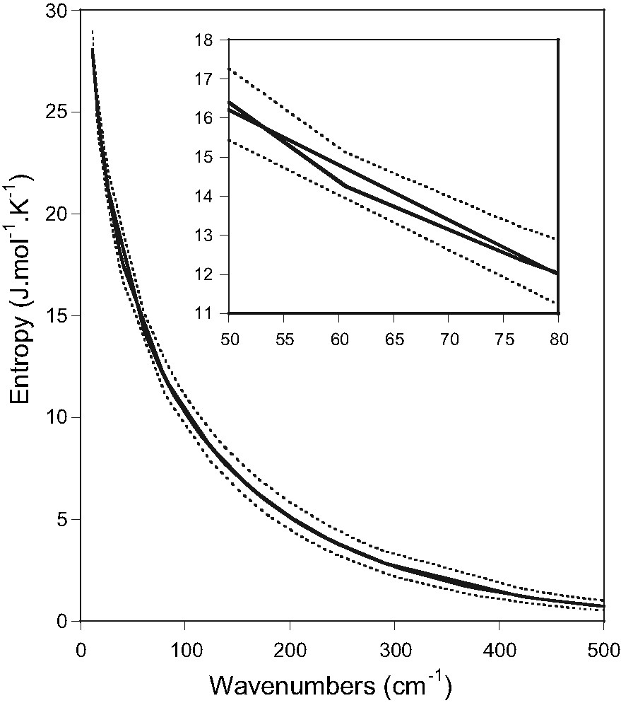
Calculated LS and HS vibrational entropies as a function of the frequency (full lines). Dotted lines represent the calculated entropy with 10% error on the vibrational frequencies.
Let us finally note that the very low frequency range (below ca. 150 cm–1) has a major contribution to the entropy change. In this frequency range the separation of lattice and intramolecular modes – inherent to the applied DFT method in which we considered only a single molecule – is a doubtful approach. Hence, calculated frequencies in this range are subject to larger errors, all the more that no isotope labeling data have been published below 100 cm–1.
4 Conclusions
We used isotope substitution technique to evaluate the efficiency of different DFT methods in estimating the molecular vibrational frequencies. We found that each computational method (B3LYP and BP86) predicts remarkably well the isotope substitution effects as far as the number of shifting peaks and the magnitude of isotope shifts are considered. Concerning the calculated frequencies, they often differ by as much as 20 cm–1 from the experimental ones, the BP86 function with the 6-311G(d) basis set being (in general) more accurate. It is worth to mention that a better agreement can not be since that measurements are done in the solid state, while calculations are carried out for single molecules. Although the frequency calculations proved to be fairly reliable, the vibrational entropy change upon the SCO was obtained only with a qualitative accuracy due to the exponential dependence of the entropy on the vibrational frequencies. Therefore, as far as the calculated frequencies are subject to – even small – systematic errors, a quantitative determination of ΔSHL by DFT calculations can only be fortuitous. On the other hand, with the possibility of assignment of normal modes, the DFT methodology remains a valuable tool for the analysis of the contributions of these modes to the total entropy change.
Acknowledgements
The authors are grateful for a European Commission Marie-Curie Fellowship (Villő K. Palfi) and the Calculs en Midi-Pyrenées (CALMIP, Toulouse, France) supercomputer center for calculation facilities.