

1 Introduction
The IPS series was born out of the perceived crisis in oil supply that followed the Arab oil embargo that was declared following the 1973 Arab–Israeli war. The first symposium (designated by the number 0) was organized by Prof. Norman Lichtin to try to redirect the various directions that photochemistry was taking (designated by the conference as Photo-Inorganic, Photo-Organic, Photo-Biochemical and Photo-Electrochemical) toward a well-defined societal objective, namely, an increase use of solar energy as an energy source.
The 1973–1974 ‘crisis’ came and went—as judged by the evolution of oil prices since then. The present IPS meeting is ~15, an interval of about 30 years. From the scientific perspective the conference series has been a great success, but fossil fuels still constitute more than 90% of our energy menu. The societal issue that has emerged recently is not shortage in supply, but rather excessive use that will have direct impact on global climate through anthropogenic chemical modification of the atmosphere.
This paper is an attempt to try to refocus attention to this societal issue through the reexamination of the same remedies that were examined in the 1970s to address the supply issue.
We will start by presenting the three experimental observations that relate the energy supply to climate change. We will proceed to examine the global socio-economic structure with projections for energy use and follow by examining the correlations between projections of atmospheric chemical changes and the global supply of fossil fuel. We will conclude by presenting a computer simulation “game” that examines the effects of incorporating renewable energy sources in the energy mix.
Data:
Fig. 1 shows the change in the atmospheric concentration of carbon dioxide, as measured in one particular monitoring station. Fig. 2 shows the changes in the average global temperature over the last 120 years and Fig. 3 shows the dependence of the Gross Domestic Product (GDP) per capita on the average energy use per capita.
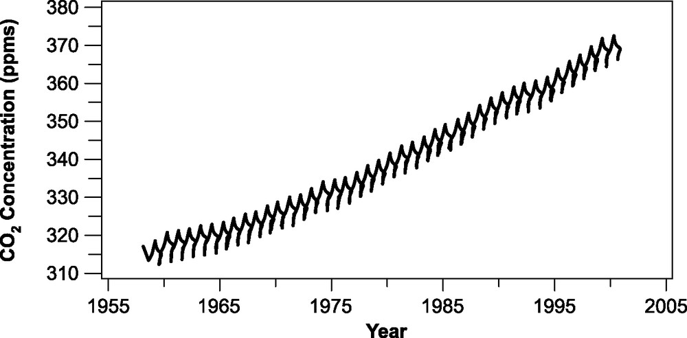
Carbon Dioxide Concentrations as observed at Mauna Loa (Hawaii) [1].
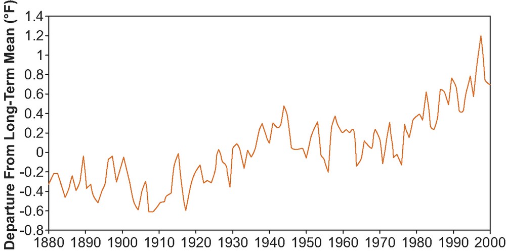
Global Temperature Changes (1880–2000) [2].
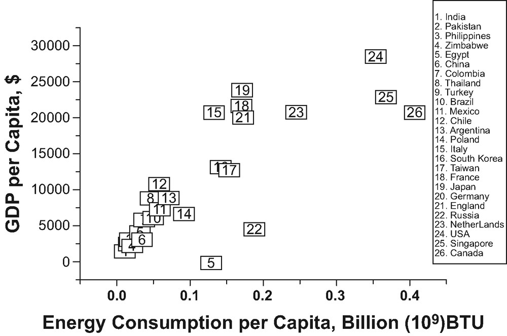
GDP as a function of energy use for various countries (Data extracted from CIA [3]).
Fig. 1 shows the atmospheric concentrations of carbon dioxide of air samples that were collected continuously from 1958. The samples are collected at Mauna Loa on the island of Hawaii. The concentration of carbon dioxide is measured by infrared absorption spectroscopy, using the same property of carbon dioxide that makes this material a greenhouse gas. The measurements show a mean yearly increase of around 17% from 1958 until today. Although Mauna Loa is the oldest site in which such measurements are made, the monitoring has expanded to different sites at different latitudes. The pattern of a monotonic increase in the carbon dioxide concentration is reproduced in every site.
Fig. 2 shows the U.S. National Climatic Data Center's (NCDC) long-term mean temperature data for the Earth, obtained by processing data from thousands of world-wide observation sites on land and sea for the entire period of record of the data. The whole Earth's long-term mean temperatures were calculated by interpolating over uninhabited deserts, inaccessible Antarctic mountains, etc. in a manner that takes into account factors such as the decrease in temperature with elevation. Similar results are reported by other agencies such as NASA [4]; the sources and the extrapolating methods appear to be the same.
Fig. 3 shows the relationship of the Gross Domestic Product (GDP) per person with the energy consumption per person for various countries in the world. The data for this figure were taken from the American's CIA database that includes a detailed collection of data for all the countries in the world. Here again, very similar data can be extracted from the World Bank's [5] database and various national energy agencies. Almost all the data are supplied by the individual countries.
If we look at the over all trend, the GDP per person increases linearly with the energy use per person until about $25 000/ person when it saturates. After that, further energy use does not result in a GDP increase. There is also great deal of scatter in the graph.
While the temperature increase on such a short (compared to geological time) time scale can be easily attributed to result from normal fluctuations of astronomical origin that have nothing to do with anthropogenic contributions, the increase in carbon dioxide concentrations and other greenhouse gases can not. There is no precedent to such an increase and independent measurements of isotopic composition have clearly established that the burning of fossil fuels is the major source of the increase. The correlation between the increase in atmospheric concentrations of greenhouse gases and the global temperature change is calculated through the concept of Radiative Forcing defined as: Change in the net radiation at the top of the troposphere occurring because of a change in concentration of atmospheric components or solar insolation.
Table 1 shows [6] the changes in the atmospheric concentrations of some of the most important greenhouse gases and their corresponding Radiative Forcing. Positive Radiative Forcing implies adjustment through an increase in average global temperature. Computer modeling compiled through the IPCC efforts [6] predicts an average global temperature rise of about 2.4 °C as a result of doubling of the CO2 atmospheric levels.
Preindustrial and present atmospheric concentrations of the major greenhouse gases
| Greenhouse gas | Preindustrial Concentration | Atmospheric Concentration | Radiative Forcing |
| In ppbv | In 1994 in ppbv | In W/m2 | |
| Carbon Dioxide | 278 000 | 358 000 | 1.46 |
| Methane | 700 | 1721 | 0.48 |
| Nitrous Oxide | 275 | 311 | 0.15 |
| CFC-12 | 0 | 0.5 | 0.17 |
Some data on global use of fossil fuels and the resulting carbon dioxide emission that will find further use are also given in Table 2.
Data for global energy use and emission in 1999 (Based on data from the World Bank [5])
| Energy use (Btu) | 3.8 × 10¹⁷ (0.38Q) |
| Carbon Dioxide Emission | 6.1 Gt-C |
| Change in the atmospheric concentrations due to addition of carbon dioxide | 1 ppmv = 1.5×10¹⁴ moles of carbon = 1.8 Gt-C |
2 Dimensional analysis
Efforts to ‘predict’ the climatic consequences as a result of given set of emission scenarios are predicated on the modeling of the anthropogenic contributions to future climatic trends. These efforts are now being coordinated by the Intergovernmental Panel on Climate Change (IPCC) [6]. The political coordination is still a work in progress. The models start with a scenario for socio-economic projections that assume certain values for population growth, changes in GDP (Gross Domestic Product) and GDP distribution, and total energy use and energy mix. From these data, the quantity of greenhouse gases (GHG), emissions are estimated. The dynamics of the distribution of the GHG between air, land and oceans are modeled and future atmospheric concentrations of the GHG estimated. Based on present estimates of the radiative forcing of these gases, the future increase in the average global temperature can be estimated. This estimate of the average global temperature can be translated into terms such as potential rise in sea level and local changes in the frequency of weather extremes.
3 Separation of variables
The essential role that both socio-economic human factors and the science of the physical environment play in modeling future climate changes makes the issue very complex. A method was proposed in the 1970's to simplify the issue by formally presenting the increase in greenhouse gases as a product of various factors in such a way that the dimensions of the various terms cancel out. This kind of analysis is referred to as ‘dimensional analysis’. In the context of environmental issues, this methodology is known by the acronym of IPAT [7–8] where I stands for Impact, P for population, A for affluence and T for Technology.
For emission of CO2, the identity can take the following form:
| (1) |
The impact here is the environmental impact (CO2/Year) and GDP/Population (or as it is more often expressed as GDP/Capita) is the measure of Affluence. The rest of the terms refer to the Technology part of the acronym. The next term describes an issue that is often referred to as energy intensity. For a given population change, the policy goals are to minimize CO2 production while at the same time maximizing the GDP/capita.
Fig. 4 shows the median estimate of the growth in world’s population [9]. It estimates that toward the second half of the 21 st. century, the world’s population will stabilize at around 9 billion people. The forces that will drive this stabilization include an increase in the standard of living (as measured by GDP/Capita) and, in particular, the increase in the education level (and the decision making) of women in developing countries. The next term in Eq. (1) is the GDP/Capita. One of the global statistical classifications that the UN employs [9] is to divide the countries of the world into three income categories: high, middle, and low income. The average world GDP/Capita and those of the three categories are shown in Table 3. The high-income category constitutes of 56 countries with GDP/Capita > $9000. These include the countries in Western Europe, North America, Japan and Australia. The Middle Income countries are 88 countries with $735 < GDP/Capita < $9000. Some of the largest countries in this group are China, Egypt, Brazil, and Turkey. The Low Income Countries are 64 countries with GDP/Capita < $735, including India, Nigeria, Pakistan, among others.
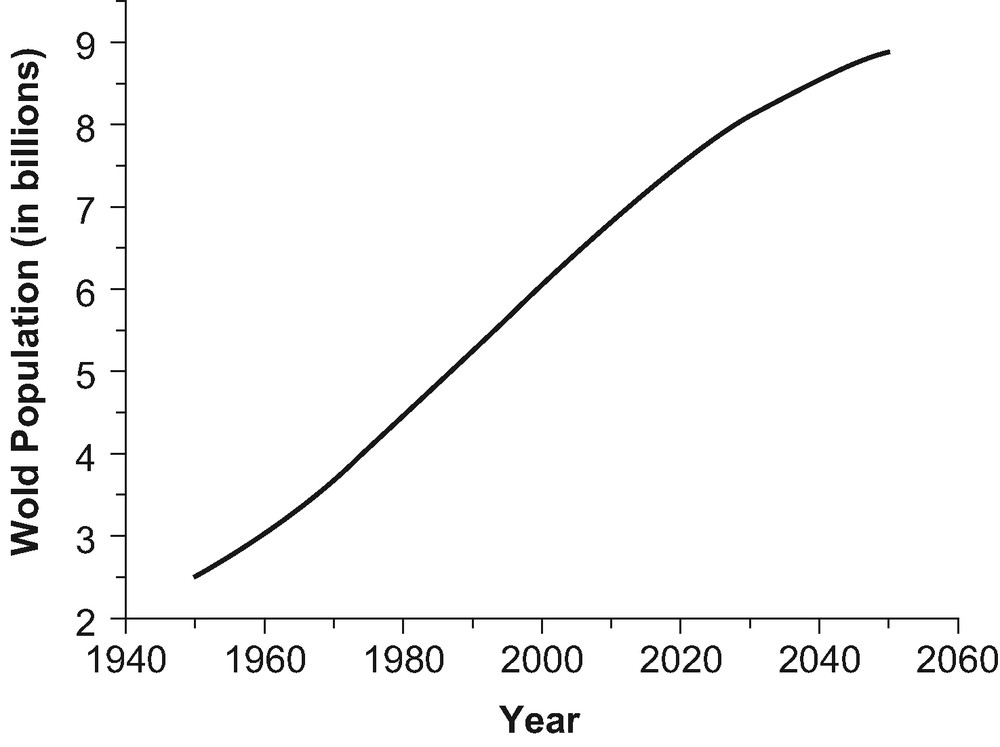
UN Median Estimate of the World Population [9].
Global income groups and mean GDP/capita
| GDP/Capita, US$ | |
| World | 5210 |
| High Income | 26900 |
| Low Income | 452 |
| Middle Income | 1870 |
The average world GDP/Capita is $5210. The policy objectives of the UN and other international organizations to raise the GDP/Capita of the developing countries to the level of that of the developed countries implies raising the average global GDP/Capita by a factor of 5.2, assuming no change in the standard of living of the developed world. Assuming that everything else in Eq. (1) remains constant, and using the 1999 levels of global carbon dioxide emission, such an increase in the global standard of living will result in yearly emission of CO2 to a level of 31.7 Gt-C to the atmosphere (compared to 6.1 Gt-C in 1999, see Table 2). Assuming that about half of that emission stays in the atmosphere and the other half enters the carbon cycle to equilibrate with the Oceans, about 16 Gt-C will remain in the atmosphere resulting in an increase of 9 ppmv/year in the atmospheric concentration of carbon dioxide. This level will very quickly double the atmospheric concentration of carbon dioxide compared to the pre-industrial levels which, following IPCC [6] compiled conservative modeling estimates, will result in a 2.4 °C increase in average global temperature. The term that follows the GDP/Capita in Eq. (1) is the energy/GDP term, known as energy intensity. Fig. 3 shows that this term is approximately constant, that is, independent of the standard of living of the countries. At the end of this paper we will show how important this term is for scenarios of the global energy future. The rest of the terms in Eq. (1) relate to the energy use and will be addressed in the computer modeling of various energy scenarios explored toward the end of the paper.
The hidden term that does not show explicitly in Eq. (1), but which has a profound effect on the energy (technology) terms in the equation, is the supply of fossil fuel. Do we have enough fossil fuel to feed global need to raise the global GDP/Capita by a factor of five in a sustainable way, keeping the other terms in the equation constant?
Table 4 shows the ‘proven’ reserves of conventional (oil, natural gas and coal) fossil fuels in 2002. The last column in this Table is marked as R/P (reserves/yearly production). This ratio approximately indicates the number of years that the reserves will last at current production levels.
Proven ‘Conventional’ World Fossil fuel reserves – 2002 [10]
| R/P, Years | ||
| Oil (billion barrels) | 1050.3 | 40.6 |
| Natural gas (trillion cubic feet) | 5501.5 | 60.7 |
| Coal (Mtons) | 984 453 | 204 |
We expect that oil and natural gas will last about 50 years and coal about 200 years.
The issue of a finite oil supply and its effects on human development is not new. M. King Hubbert, at the time a geophysicist at Shell, was trying to develop oil forecasting techniques for the oil industry as early as 1969. The result was a bell-shaped curve that bears his name, similar to Fig. 5 [11].
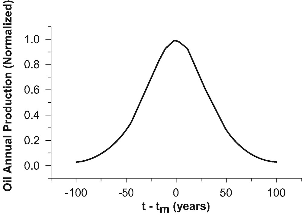
Schematic presentation of the Hubbert Peak.
The maximum production rate from US reserves was initially predicted to take place in the mid-1960s and was extended later to the beginning of the 1970s. Comparisons of forward productions with actual productions could be matched well after minor adjustments in the curve. It is not surprising that the Hubbert peak gave rise to the Olduvai Theory [12] in which industrial civilization will decay around 2025.
The Hubbert peak and its derivatives are all based on limited supply. The future of fossil-fuel-induced climatic changes is based on availability. Table 5 shows an estimate of ‘ultimate’ fossil fuel energy reserves. Again, the estimate of ‘ultimate’ should be regarded with some suspicion.
‘Ultimate’ energy reserves [10]
| Fuel | Amount | Energy | Carbon |
| (Q = 1018 BTU) | (1011 tons C) | ||
| Oil | 2000 Gbrl | 12 | 2.7 |
| Natural Gas | 1016 Ft3 | 10 | 1.5 |
| Coal | 8 × 10¹² tons | 210 | 80 |
| Oil Shale | 3 × 10¹¹ tons of Oil | 3.7 | 3 |
| Tar Sand | 3.5 × 10¹¹ barrels of Oil | 2.1 | 1 |
| Methane Hydrate | 2.5 × 10²⁰ Ft3 | 250 000 | 37 000 |
The values here are normalized to common energy units and the amount of the released carbon. The conclusion from these numbers is very clear and seems to be robust enough to withstand the softness of the numbers in the table: Assuming that the present equilibrium in the carbon cycle is not disturbed and that only about 50% of the released carbon dioxide stays in the atmosphere, oil and natural gas will add ‘only’ 100 ppmv to the atmosphere. Such an increase is currently modeled to raise the average global temperature by about 1 °C. If coal, oil shale, and tar sand are added to the mix, the added carbon dioxide could increase atmospheric concentrations by as much as 2500 ppmv. Such an increase could raise the average global temperature by as much 10 °C and will open the possibility of a Venusian fate. The use of methane-hydrate, development of which is already in progress at number of sites, opens the possibility for a much faster time scale to reach such a fate. The R/P values given in Table 4 provide us with a time of about two generations to reach a policy decision that will prevent such an occurrence.
4 The energy game
A computer ‘game’ was created both as an educational tool to demonstrate the complex interactions of the various socio-economic forces mentioned in the previous section, and as a tool that might assist in generating credible scenarios for global sustainable development.
4.1 The ‘world’
An input population with different GDP/capita is constructed to model the world’s countries. An example of such a population is shown in Fig. 6.

Schematic representation of the ‘world’ that plays the ‘energy game’. The area of the circles is proportional to the initial wealth of the countries as measured by GDP/capita.
The size of the GDP is proportional to the area of the circles. The initial GDP ratio between the richest and the poorest countries is 10.
4.2 The rules
Initially the population consists of a quarter rich, a quarter poor and half with an intermediate standard of living. If we designate the GDP of the poor countries as 1, at each time step, the population of the ‘world’ increases subject to the following criteria:
GDP < 1 4%
1 < GDP < 3 3%
3 < GDP < 5 2%
5 < GDP < 7 1%
7 < GDP 0%
The ‘world’ is connected to two energy sources: fossil fuel and renewable sources. For this game, nuclear energy is considered renewable because its economics and the climatic consequences at issue here are similar to solar energy. The price of the energy from these sources varies in the following ways: The price of the fossil fuel increases as the reservoir is depleted and the price of the renewable source decreases with the amount used, reflecting the notion that a significant fraction of that price goes to initial capital investment that gets amortized with the amount of energy used. Specifically, the price structure follows the following relation:
| (2) |
| (3) |
At each time step, every ‘country’ buys the least expensive energy and the GDP of the country changes following the following rules: 50% is ‘wasted’ on consumption and additional 10% goes to saving; since we are not doing here anything with the saving, this additional 10% also counts as consumption. What is left is spent on purchasing energy. The energy that is bought is used to create more GDP according to the stipulated energy intensity, assumed to be independent of GDP. When a ‘country’ splits according to the corresponding growth statistics, the GDP is equally divided between parent and ‘daughter’.
5 Results
Figs. 7 and 8 show typical results of a run. The time period chosen here is 70 years, which approximately corresponds to the life span of three co-existing generations (i.e. grandparent to grandchildren). The span also approximately agrees with the R/P values for oil and gas previously mentioned. In both figures, we compare the time evolution of the GDP/Capita and the paid price of energy with and without the use of renewable energy resources under three different energy intensities. The figures clearly show that without sustainable, renewable energy sources, the sharp decline in oil supply leads to the derived increase in the price of energy and the resulting decrease in GDP/Capita, predicted by Hubbel. However, the results also show the key role that energy intensity plays in the balance. Based on the very simplistic scenario and the given set of initial conditions, high energy intensity results in an immediate drop in GDP/Capita and relatively low energy consumption as a result of inability to pay higher prices. Low Energy Intensity, on the other hand, initially generates enough GDP to pay for much higher energy prices and thus will initially lead to a considerable higher GDP/Capita and higher energy use, even without the inclusion of renewable energy in the available energy mix. However, regardless of the energy intensity, absence of renewables in the energy mix will inevitably lead to the Hubbert decline. Inclusion of renewables in the balance changes this picture drastically. At high-energy intensity, there is at first an increase in the standard of living followed by a decline due to the inability of the economy to generate enough GDP to pay for additional energy. At low intensity, on the other hand, the price of energy eventually drops to the lowest price for renewables allowed by the model and the GDP/Capita continues to rise fueled by a complete energy shift to renewable energy sources. Limited experimentation with the game did not allow us to determine if stable steady-state solutions are possible within this model, but the game is being developed further to explore its scope.

The time evolution of the GDP/Capita at three different energy intensities. The GDP/Capita is normalized to the initial GDP/Capita of the poorest countries. The time is expressed in number of years after the present time.
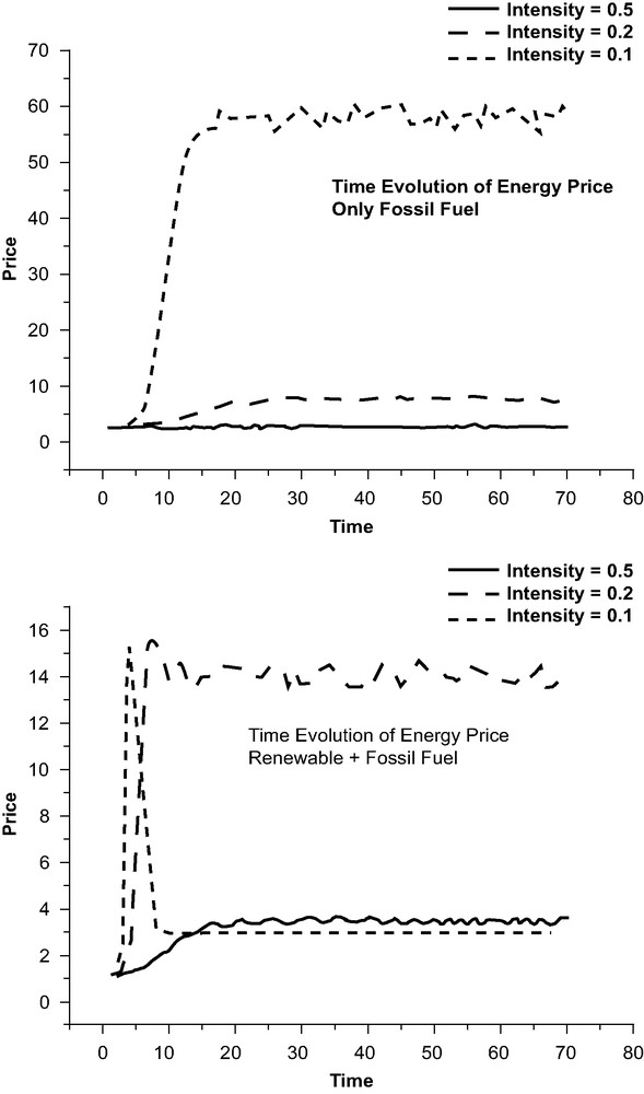
The time evolution of the price (normalized to initial cost) at three different energy intensities.
6 Conclusions
The socio-economical projections and the estimated fossil fuel reserves show that a continuous reliance on fossil fuel for global energy supply will produce major climate-induced ecological changes within 2–3 generations. The simulations strongly suggest that a commitment to renewable energy sources such as the ones derived from solar energy can ensure an energy supply without the adverse climatic consequences. Some of the questions that remain unanswered focus on issues of the sensitivity of the global economy to the price crossover between fossil fuels and the alternative energy sources.