Retrieving accurate relaxometric information from low signal-to-noise ratio <sup>23</sup>Na MRI performed in vivo

Mihaela Lupu; Carole D. Thomas; Joël Mispelter

doi:10.1016/j.crci.2007.09.007

Résumés

Anglais
Français

Sodium is the second best nucleus in living systems MRI after proton, but it is the first one concerning its sensitivity to the electrical configuration of the environment, due to its quadrupolar relaxation properties. Retrieving accurate relaxation data from low signal-to-noise ratio (SNR) experiments implies using post-processing procedures in order to fit correctly the decaying relaxation curves. The conventional image reconstruction method is introducing a positive bias due to the rician noise contribution. Phasing the images restores its initial Gaussian characteristic. Linear prediction (LP) forward of the decays improves the SNR of the last points and calculates missing points. An objective fitting method, based on singular value decomposition (SVD) allows us to determine the number of exponentials existing in the decay and its accurate fitting parameters. Sodium ions' spin–spin relaxation holds great potential to become an endogeneous marker for tumor diagnosis and for therapy response, since different regions of a mouse tumoral liver bear distinguishable relaxation parameters as compared to control.

Après le proton, le sodium est le second noyau abondant observable par RMN dans les systèmes vivants. Il est aussi le plus sensible à l'environnement grâce à ses propriétés de relaxation quadrupolaire. Une relaxométrie précise requiert cependant, pour un noyau peu sensible comme le sodium, de préparer au mieux les données acquises avant toute tentative d'exploitation. Les images sont d'abord reconstruites en mode phasé, évitant ainsi le biais induit par le redressement du bruit caractéristique de la reconstruction en mode valeur absolue. Une prédiction linéaire progressive permet ensuite de propager le meilleur rapport signal/bruit des premiers points vers les plus tardifs et de prolonger le déclin, si nécessaire. Cela permet d'utiliser une méthode objective et quantitative de décomposition des déclins en multiexponentielles, basée sur la SVD. Un exemple est donné, montrant la sélectivité de la relaxation spin–spin du sodium pour deux régions, saine et tumorale, du foie de la souris. La relaxation spin–spin des ions sodium constituerait ainsi une sonde endogène pour le diagnostic et le suivi thérapeutique de tissus tumoraux.

1 Introduction

In research studies or in clinical investigations, images are used not only for evidencing the inner structures of the body but also for quantifying the available NMR parameters, like T₁, T₂ or the apparent diffusion coefficient, D. Especially, T₂ evolution on the treatment time-course is more and more considered as a possible early apoptosis marker, hence an important NMR parameter to be taken into consideration in research or in clinical treatment [1,2].

In these conditions, the accurate determination of the relaxation time constants characteristic for targeted tissues, determined from a specific region of interest (ROI) on the reconstructed image becomes of major importance. Moreover, the complexity of the molecular motions leading to the nuclear relaxation in biological systems confers multi-exponential characteristics to the investigated systems. The need to quantitatively determine the relaxation time constants from non-exponential decays leads to some mathematical manipulations in order to extract more accurately the transformed signal amplitudes. All these reasons imply a certain degree of accuracy when relaxation calculations are performed using MRI data, close to the requirements usually encountered in spectroscopic techniques.

But what has become obvious in spectroscopy and almost unnoticed, becomes cumbersome and difficult when data are retrieved from images amplitude. The post-acquisition data processing proposed here implies phase correction of the reconstructed images, smoothing the retrieved decay curves by linear prediction – forward and fitting by the singular value decomposition method.

1.1 Phasing the images

The great majority of reconstruction methods implemented on the imaging machines are using the absolute amplitude of the FFT coefficients of the recorded signals, in order to obtain the final image. This method is simple to implement and has the great quality of avoiding the necessary phase corrections (used in spectroscopy). The absolute value reconstruction method uses the pair of images representing the real and imaginary components of the FFT transform to calculate the magnitude, I, of each corresponding complex pair:

I = \sqrt{{Re}^{2} + {Im}^{2}}

This calculation, performed for every point in the reconstruction grid, has the undesired effect of biasing the noise level to a certain positive value, as presented in Fig. 1. This type of “noise” has lost its Gaussian characteristic (carried by the acquired echoes), becoming rician.

Fig. 1
Rician noise (left), after absolute value reconstruction method, showing a positive bias around 1.5 (arbitrary units). Gaussian noise (right), after phase correction procedure, the same carried by initial signals, prior to the reconstruction. Notice the null average of the noise in this case.

This positive bias increases as the SNR decreases or as the nuclear sensitivity of the resonant nuclei decreases, as it is the case for sodium MRI. The presence of the positive bias level is affecting the accurate determinations of the NMR relaxation parameters such as T₁, T₂ as well as any result of pixels algebra. Nevertheless, even in the case of high SNR proton images, multi-exponential relaxation may be covered up by the positive noise level. So far, a few attempts were done to overcome the noise problem of the reconstructed images in MRI.

The use of power magnitude values, I² [3] is reducing the noise effect over the region of interest, allowing the substraction of noise contribution. However, this power routine is only valid for exponential relaxation decays, while most of the biological samples are heterogeneous and thus non-exponential.

Another way to avoid the undesired biased noise produced by magnitude calculation is to phase-correct the images. If real, phase-corrected images are to be produced, they have the advantage of preserving the same noise characteristics as the original acquired signals. Ideally, the phase correction is achieved by rotating all the FFT coefficients in the complex plane, such that all information are transferred to the real component while the imaginary one tends to zero (noise level). An attempt to obtain phase-corrected images was done by van der Weerd et al. [4]. Their algorithm is based on the phase calculation of every pixel for the first and second echo images and the resulting correction is then applied for all echoes in the sequence. The first two echoes are thus becoming magnitude images while the rest of echo images are real, phase corrected ones. Nevertheless, when extracting the decay curve from the whole echo images train, a small bias is introduced for the first two points, characterised by the highest SNR values in the sequence.

Ideally, one should phase-correct all the images, using all available, acquired information. We have developed a novel and accurate method for phase correcting all images, by phasing each pixel separately, using all the echo images available in the sequence [patent pending]. The phase correction procedure is briefly shown in Fig. 2. Following the FFT procedure, the echo decays represent a mixing of real and imaginary intensities, as shown in Fig. 2a. The phasing procedure acts on each pixel of the images in order to maximise the real intensities while minimising the imaginary ones. Following the phase-correction procedure, the real phase-corrected images are obtained, allowing the retrieval of corrected amplitudes for the decay curves, Fig. 2b.

Fig. 2
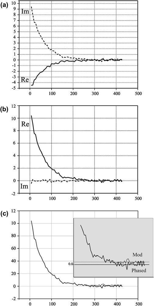
The effect of phase correction procedure on the relaxation decay of a solute NaCl sample: (a) the complex relaxation decay as obtained from a multiple spin–echo imaging experiment; (b) following the phase correction procedure, the real part of the decay is maximized, while the imaginary part tends to null, and (c) the difference between the phased decay and the absolute one is evidenced mainly for the last echoes, where the noise becomes increasingly important in SNR.

The phasing procedure applied on the spin–spin relaxation decay is shown in Fig. 2c, as compared to the absolute value decay. As expected, the phase corrected decay tends to the Gaussian noise level, while the absolute value decay tends to the constant value given by the averaged absolute value of the noise. The decays correspond to a solute NaCl sample characterised by an exponential spin–spin relaxation process. The SVD fit of an exponential decay is characterised by one singular value detaching from noise, as obtained for the phase corrected decay, Fig. 3. The presence of the constant positive value for the absolute decay induces a second singular value detaching from noise, indicating completely erroneous biexponential decay for the same sample.

Fig. 3
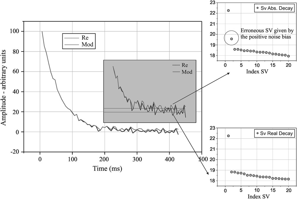
Phase-corrected and absolute value decays of a solute NaCl sample and their corresponding singular values detaching from the noise. The modulus decay tends to a positive value while the phase-corrected decay tends to null. The positive bias gives an erroneous second singular value when the corresponding decay is subjected to SVD.

The procedure allows both the accurate T₂ determination for any ROI defined on an image obtained by a multiple-echo experiment, like multiple-slice multiple echoes (MSME), and correct image algebra, if required. We have applied the phase correction routine on sodium images, characterised by rather poor SNR values, in agarose-gel samples as well as in vivo mouse liver. The exponential decays thus obtained were fitted using the singular value decomposition method in order to obtain objective fitting parameters.

1.2 Data analysis

The relaxation decays retrieved from the MSME images are expected to represent a sum of, at least, two exponentials:

S (t) = A_{1} \exp (- \frac{t}{T_{2short}}) + A_{2} \exp (- \frac{t}{T_{2long}}) + noise

where A_i are the corresponding amplitudes characterised by the two time constants T_2short and T_2long. Such curves were analysed using the singular value decomposition (SVD) fitting method. This fitting method provides, on the one hand, an objective criterion regarding the number of exponentials present in a decay curve, and yields, on the other hand, a criterion about the data accuracy, as it is sensitive to noise level [5].

The data points, {s_i} obtained from the T₂ decay are rearranged in a matrix form having a Hankel structure:

H = (\begin{matrix} s_{0} & s_{1} & \cdot & \cdot & s_{q - 1} \\ \cdot & \cdot & \cdot & \cdot & \cdot \\ \cdot & \cdot & \cdot & \cdot & \cdot \\ \cdot & \cdot & \cdot & \cdot & \cdot \\ s_{p - 1} & s_{p} & \cdot & \cdot & s_{p + q - 1} \end{matrix}); H_{i, j} = s_{i + j - 1}

Such matrices are easily factorised using the SVD theorem:

H = U Σ V^{T}

, where U and V are orthogonal and Σ is diagonal. We obtained thus the singular values (the elements of Σ) that are directly related to the exponents involved in the decays [5]. This method is stable and reliable, and offers, in an objective way, the number of exponentials present in the experimental decay, corresponding to the number of singular values detaching from noise level. The singular values characterising the signal are subjectively detected by the “jump” from the noise's singular values. The jump is obvious for very good SNR values but an “operator-free” criterion is given by Lin et al. [6].

The requirements for using the SVD analysis of a decay curve are a constant sampling of the decay and the total description of the curve up to noise level. The noise plays an important role in this analysis since it represents the limit for the rank detection of the Hankel matrix. This objective fitting method depends on the Gaussian, unbiased noise level, since every data point is carrying the additive information regarding both the pure signal and the noise existing along the detection channel. In order to make clear the role of the noise in the SVD algorithm, we simulated several biexponential decays, similar to those determined for sodium in living tissue (liver) [7]. Hence we generated a sum of two exponentials (with time decays and amplitudes close to experimental values) for which the noise level was increased up to a level where the fitting started to be erroneous and the singular values were no longer detached from noise. Fig. 4 shows the detection of the two singular values characterising the biexponentiality of the simulated decay as a function of the noise level. The SNR factor is defined as [6]:

SNR = \frac{S (t_{0})}{2 σ_{noise}}

where S(t₀) represents the total amplitude for the first echo-time and σ the noise standard deviation. For the lowest SNR values (14, 20), only the first SV is rising noticeably above the noise level. The second SV becomes obvious for the SNR values above 40. It is obvious that imaging experiments are time limited since the animals are generally under anaesthesia during the measurements. In practice the accumulated SNR (1.5 h), generated by the MSME sequence was in the range 20–40, depending on the tissues' sodium concentration. Table 1 presents the results of SVD fit as a function of the SNR level.

Fig. 4
Dependence of the first six singular values amplitudes as a function of SNR of the simulated biexponential decays, before applying the LP procedure. Only for SNR = 80, the second singular value is detaching from noise.

SNR	T_2long (ms)	T_2short (ms)	A_long	A_short	Chi-square
14	28.7	16.5	1896	200	0.885
20	28.9	16.2	1884	226	0.87
40	34.8	10.6	1491	765	0.792
80	35.1	10.7	1476	767	0.78
Simulated	35	10	1500	750	–

Chi-square values are defined as [8]:

χ^{2} = \frac{\sum_{i} {(s {(i)}_{calc} - s {(i)}_{exp})}^{2}}{(n - 1) σ_{noise}}

For the lowest SNR, when fitting with a biexponential, the results become erroneous, independent of the chosen fitting method. The chi-square values, dependent on the SNR, represent an indication of the fit accuracy.

In order to increase the fitting accuracy we had to smooth the data. Again, unlike the spectroscopical CPMG sequence, the MRI inter-pulse distance is limited as well as the number of echoes due to the power deposition condition. For small animal imaging, the number of echoes may vary between 16 and 32, for clinical investigation usually being less. It is obvious that usual smoothing routines (interpolation, average) that are successfully applied in spectroscopy for 200–300 echoes cannot be applied here, since we cannot afford losing any data point information. A simple and quite satisfactory smoothing routine is based on linear prediction theory.

1.3 Data smoothing using linear prediction —forward

Usually, the linear prediction procedures are used in spectroscopy as a replacement of FFT procedure, in order to fully determine the characteristics of a dumped sum of sinusoids (frequency, phase, amplitude and width at half height) [9,10].

The mathematical model for NMR signals (i.e. the periodic, time-dependent free induction decay or exponential decay) is nonlinear. The nonlinearity can be circumvented by invoking the principle of linear prediction (LP) modelling that assumes that each data point can be expressed as a linear combination of a set of M consecutive data points. Using M previous data points to calculate subsequent ones is called forward linear prediction since the prediction is forward in time:

s_{n} = \sum_{i = 1}^{M} f_{i} s_{n - i}

M is called the order of prediction and the above equation may be applied N − M − 1 times, where N is the total number of available data points. Using M data points to calculate previous ones is called backward linear prediction since the prediction is backward in time:

s_{n} = \sum_{i = 1}^{M} b_{i} s_{n + i}

It is obvious that both forward and backward prediction estimates are linear combination of the same observable data, but their effect on calculated points is different and deserves some comments.

Usually, linear prediction is used to extend in time insufficient collected signals in both directions [7]. This is the case for missing points at the beginning of the acquisition array due to the spectrometer dead-time or rather long echo-time or at the end of the acquisition array for missing data towards null. The backward LP completes missing points at the beginning of the acquisition array, while forward LP completes missing points at the end.

A “side effect” of the LP is noise cleaning, since the experimental data are digitally reconstructed using the first data points having the highest signal-to-noise ratio.

The following example illustrates the use of forward linear prediction routine. First, six linear predictors f₁ … f₆ are calculated using a linear system of, for example, 10 equations as below.

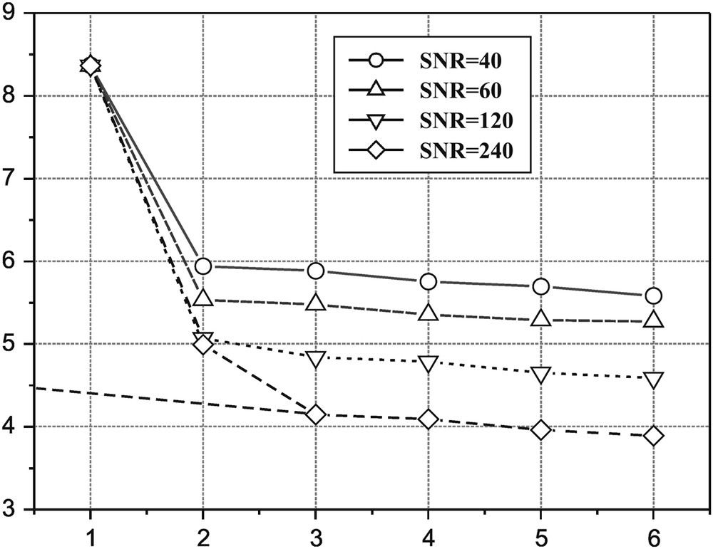
{\begin{cases} s_{7} = f_{1} s_{6} + f_{2} s_{5} + f_{3} s_{4} + f_{4} s_{3} + f_{5} s_{2} + f_{6} s_{1} \\ s_{8} = f_{1} s_{7} + f_{2} s_{6} + f_{3} s_{5} + f_{4} s_{4} + f_{5} s_{3} + f_{6} s_{2} \\ s_{9} = f_{1} s_{8} + f_{2} s_{7} + f_{3} s_{6} + f_{4} s_{5} + f_{5} s_{4} + f_{6} s_{3} \\ s_{10} = f_{1} s_{9} + f_{2} s_{8} + f_{3} s_{7} + f_{4} s_{6} + f_{5} s_{5} + f_{6} s_{4} \\ \cdot \\ \cdot \\ \cdot \\ s_{16} = f_{1} s_{15} + f_{2} s_{14} + f_{3} s_{13} + f_{4} s_{12} + f_{5} s_{11} + f_{6} s_{10} \end{cases}

Using the linear predictors thus obtained, all decay data are recalculated starting with index 7. In our example the “last” experimental data point used for smoothing is s₆, so the noise carried by it will propagate through all calculated points.

The effect of forward linear prediction procedure on the SV levels is quite impressive. Fig. 5 shows again the dependence of SV (for the same generated curves as in Fig. 4), after performing the LP procedure.

Fig. 5
Dependence of the first six singular values amplitudes as a function of SNR before (dotted grey) and after (black straight) LP procedure. We used here six linear predictors and 10 linear equations for all cases. The singular values that characterise the noise level are lower for the LP treated data, allowing the rise of the second singular value characterising the biexponential decay, starting with SNR = 20.

Firstly, the singular values characterising the noise level are lowered by the linear prediction procedure, for all SNR cases. Consequently, the second SV rises above the noise level for the SNR = 40 case, becoming noticeable. Secondly, the procedure greatly improves the fitting results, especially for lower SNR cases (Table 2).

SNR	T_2long (ms)	T_2short (ms)	A_long	A_short	Chi-square
14	31.7	6.72	1752	691	0.822
20	33.1	9.0	1619	705	0.81
40	34.3	10.3	1525	728	0.697
80	34.8	10.2	1499	749	0.69
Simulated	35.00	10.00	1500	750	–

A crucial point on using a LP procedure is the choice of the number of the predictors and the number of equations used for calculation [10]. On the one hand, these numbers will impose the quantity of noise carried through the signal. On the other hand, increasing the number of predictors (and equations) increases the accuracy of prediction too. There is an optimum, depending on each particular case that should be looked for.

When processing very low SNR systems, the number of predictors should be larger than the number of exponentials expected to be present in the decay. For our study, taking into consideration the lowest SNR, we used six predictors and 10 linear equations.

Table 2 presents the fitting results on the noisy simulated decays (as in Table 1), after linear prediction – forward smoothing.

It is interesting to notice that the most beneficial LP treatment is obtained for the lowest SNR curves, for which the fitting results as well as the chi-square values are improved.

2 In vivo T₂ relaxation results on mouse liver

In vivo experiments were performed on 17 nc/z female mice, normal and tumoral (Institut Curie breeding facility), on a Bruker Biospec system operating at 4.7 T. The RF coil was a home-made sodium (quadrature), proton (linear) birdcage coil, operating at 53/200 MHz. Single slice, multi-echo (16–32 echoes) images were recorded for sodium studies (TR = 350 ms, TE = 6.04 ms, FOV = 6.8 cm, matrix 64 × 64, slice thickness 6 mm) using 160 averages. Firstly, the images were phase corrected in order to avoid the rician noise created by modulus reconstruction. The Na relaxation curves, measured in regions of interest (ROI), were forward linear projected in order to reduce the noise amplitude and to reach the base line, required for a proper multi-exponential SVD fitting. Error estimations were performed on 100 runs by Monte Carlo simulations.

Fig. 6 shows the sodium MRI results obtained on a tumoral mouse liver as compared to control. ROI₁ is a chosen area in the liver tumor, while ROI₂ is chosen in the normal tissue. The sodium contrast is principally due to the changes in local cellular organization. Due to the quadrupolar characteristics of sodium ions relaxation in biological systems, the electrical changes of the environment are immediately reflected on its relaxation parameters. Generally, tumors are characterised by loose cellular packing, especially at the centre, where necrotic regions are developing. The necrotic regions are not empty spaces, but are full of extracellular juice of Na ions at 140 mM concentration. These circumstances allowed us to distinguish different areas in the liver. A biexponential fit of the decay could be obtained in the tumoral region due to the specificity of sodium ions relaxation and to the locally increased SNR. In the normal region, the decay appears monoexponential due to the following reasons. Firstly the cellular packing is more compact, allowing less extracellular space and consequently the fast relaxing component T_2fast is expected to be close to the detection limits imposed by the time delay between the pulses of the CPMG sequence. Secondly, the total sodium content of the tissue is expected to be decreased, resulting in a lower SNR, preventing the second SV to rise above the noise level.

Fig. 6
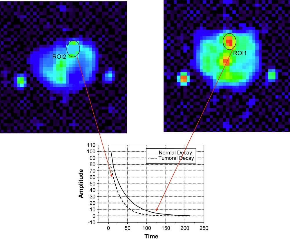
Normal (left – ROI₂) and tumoral (right – ROI₁) liver sodium images and the corresponding relaxation curves obtained from the two ROIs shown in figure. The images show an endogeneous sodium contrast for tumors (orange, yellow) as compared to normal regions in the tissue (for interpretation of the references to colour in this figure legend, the reader is referred to the web version of this article). The sodium contrast between the tumoral and normal livers is due to the changes in tissue structure as well as changes in the relaxation properties of sodium ions. The relaxation parameters are presented in Table 3. The external markers (agarose sample) are used only as positional references.

The relaxation parameters characterising the tumoral and normal tissue regions obtained after phase correction and linear prediction procedures are presented in Table 3.

ROI	T_2long (ms)	T_2short (ms)	A_long/A_short	SNR
1	39.8 ± 4.2	4.21 ± 2.2	1.78	40
2	24.78 ± 3.7	–	–	25

They are clearly distinguishable on the basis of the corresponding relaxation properties, reflecting mostly the cellular packing of the tissue.

In conclusion, the use of a spin–echoes sequence in conjunction with post-processing techniques described here allowed to evidence the multi-exponential behaviour in tumoral regions of the mouse liver where the SNR is sufficient (about 40 or greater). Sodium ions' spin–spin relaxation holds therefore a great potential to become an endogeneous marker for tumor diagnosis and possibly for therapy response due to its sensitivity to the environmental changes.

1 Introduction

1.1 Phasing the images

1.2 Data analysis

1.3 Data smoothing using linear prediction —forward

2 In vivo T2 relaxation results on mouse liver

2 In vivo T₂ relaxation results on mouse liver