

1 Introduction
The radiofrequency (RF) probe is the very heart of a magnetic resonance experiment. It is dedicated to the excitation and reception of the nuclear (NMR) or electron (EPR) spin magnetization. Although the resonant frequencies are originally very different (in the range of “radio” and “microwave” frequencies, respectively, for NMR and EPR), the probe technology tends to be similar for both kind of spectrometers, as NMR frequencies are increasing while the development of EPR in living systems is usually performed at low field. Consequently, the resonators encountered in both methodologies are sometimes designed on the same principles. This is particularly the case for the so-called “loop–gap” resonator [1].
In this paper we will shortly review some aspects of the probe technology specifically applied to the design of resonators that create a homogeneous oscillating magnetic field in the sample volume, at frequencies less than 1 GHz. These homogeneous probes are used in a great variety of magnetic resonance (MR) experiments, such as high-resolution NMR spectroscopy, solid-state NMR, low-field EPR spectroscopy and in vivo MR imaging (both electron and nuclear spin).
2 Introduction to probe technology
Basically, the probe must convert an oscillating RF current furnished by a power transmitter into an oscillating magnetic field (usually denoted B1) and, subsequently (or simultaneously in continuous wave experiments), it must convert the off-equilibrium rotating magnetization into a current that is amplified and processed by a receiver. This implies a number of conditions that define the RF probe design.
Firstly, it must be constituted of some conductive material for handling the RF currents which create an oscillating magnetic field in the nearby space around the conductors. From the Principle of Reciprocity [2], the same conductive structure is able to detect, with an equal efficiency, the processing magnetization.
It should be mentioned at this point that the magnetic field of concern here is not the one that is long-range irradiating (far field), despite the fact that the probe is frequently (and incorrectly) named “the antenna”. The energy radiated in the probe's surrounding space does not contribute to the magnetic resonance process. It contributes rather to the losses that diminish the signal- to-noise ratio, as any other processes dissipating the electromagnetic energy in the coil resistance and in the lossy sample (imperfect conductor and dielectric). These dissipation processes lead to the heating of the sample and/or the probe. An electric field is also associated with the magnetic field. Again, one should distinguish between the conservative E field and the electric field associated with the variation in time of the magnetic field (dB/dt). The latter is, in part, contained in the radiated field, whereas the former is due to the scalar potential that exists near the probe conductors. This conservative E field is proportional to the current and to the inductance of the probe conductors. It contributes also to the overall losses and sample heating. The spatial distribution of the conservative electric field component is generally different from that of the near-field magnetic component. Because it does not contribute to the magnetic resonance process, probe designers attempt always to reduce its amplitude, generally by minimizing as far as possible the inductance of the probe conductors [3]. This review being exclusively concerned with the quasi-static magnetic field of probes, the electric field distribution will be no longer discussed.
Secondly, the conductors should be arranged is such a way that B1 is perpendicular to the main static magnetic field B0. This implies some constraints on the design depending essentially on how the sample may be inserted inside the main magnet and on the B0 orientation. Furthermore, the spatial arrangement of the conductors controls the homogeneity of the RF magnetic field. In this review, we will consider only volume probes creating a homogeneous field in the space occupied by the sample.
Thirdly, the conductive structure opposes itself to the oscillating current delivered by the transmitter, due to its self-inductance. Hence, the probe reactance should be compensated using some conjugate impedance provided by capacitors. Now, the probe becomes a resonator tuned at the desired working frequency. The high impedance of this resonator must be transformed (“matched”) into the purely resistive system impedance (usually 50 Ω) in order to optimize the transfer of energy between the probe and the transmitter (or the receiver). The very basic electrical circuits of the probe are represented in Fig. 1, for the two fundamental capacitive and inductive coupling schemes.
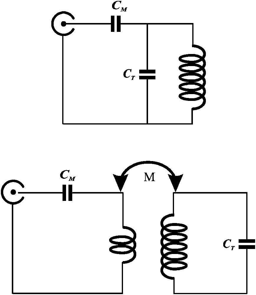
The two basic electrical circuits of a MR probe. It is constituted of a resonator (the “tuning capacitor” CT and the coil inductance) matched to the resistive 50-Ω impedance of the system by an appropriate circuit. The resonator exhibits at the resonance frequency (equal to ω0 = 1/(LC)1/2) a high, purely resistive, impedance of the order of 1–10 kΩ (Z = QLω0, typical values are: Q = 200, Lω0 = 40 Ω). Slightly out of resonance, the resistive component decreases to 50 Ω as required, but exhibits a reactive component that must be compensated for perfect match. On the lower side of the resonance, the residual reactive impedance is positive. It is compensated by the “matching” capacitor (CM), as shown in the capacitive coupling scheme (top). Another way to reduce the high resistive impedance of the resonator is to sample a small part of its magnetic flux using a coupling loop (inductive coupling, bottom). For an appropriate position of the coupling loop (adjusting the mutual inductance value M), the image of the impedance of the resonator through the flux coupling is exactly purely resistive and equal to 50 Ω at ω0. The capacitor CM compensates for the self-inductance of the coupling loop itself. Many variants of these basic circuits are found in real probes, depending on specific design constraints.
The final design should also take into account the dimensions of the probe conductors relative to the wavelength at the working frequency. A natural criterion is the product of frequency to coil diameter (fd) introduced by Doty et al. [3]. Another similar, but less direct, criterion is the coil reactance Zi at the working frequency. In practice, when fd is greater than about 20–30 MHz m or Zi is larger than 100–200 Ω, classical versions of homogeneous probes will be replaced with configurations that present less self-inductance. This is, for example, the case of the well-known “saddle” coil which is replaced at ultra high frequency (UHF) with the slotted tube [4] (or slotted cylinder [5]) configuration like in the well known Alderman–Grant resonator [6]. Similarly, the classical solenoid coil may be efficiently replaced with the scroll-coil [7] or, possibly, by the loop–gap [1,8,9].
Nevertheless, the geometry of the resonators is based on a rather limited number of designs that will be presented in the following, assuming the quasi-static approximation, i.e. after Doty [3], when the fd product is lower than 30 MHz m. The adaptation of the probe technology when the fd product increases above the limits considered throughout the paper will be shortly presented in Section 8.
3 Tools for designing and evaluating a probe
The design of a given MR probe makes use, for a large part, of previous experiences and know-how. For the beginner (and may be for the specialist too), it is very useful and more efficient to have some tools in hands in order to optimize the design, to adjust the probe component values for tuning and matching and finally to evaluate the probe after its completion.
Very expensive tools such as vector network analyzers (VNA) and highly specialized, time consuming, simulation software are normally used by professional probe designers. These tools are, however, seldom found in the MR laboratories. Fortunately, some simple rules and simple simulation tools can be usefully employed by the non-specialized engineers and, possibly, by the MR user, to learn and to understand what is under the “bonnet”.
To adjust (tune and match) a given probe resonator, one may use the “wobble” function included in most of the NMR consoles. In this configuration, the spectrometer or imager frequency is spanned around the working frequency while the energy reflected by the probe circuit, the so-called reflection coefficient Γ, is sampled and displayed on the screen (Fig. 2). When the frequency is far away from the probe resonance, all the incident energy is reflected back (Γ = 1). On the contrary, when the frequency approaches the probe resonance, part of the incident energy is absorbed by the resonator (Γ < 1) with a minimum of reflected energy at resonance, appearing as a dip in the display. If the probe circuit is perfectly matched to the spectrometer impedance (usually 50 Ω) all the incident energy is absorbed by the probe, hence Γ = 0. Such resonant spectra can be simulated by a circuit analysis software, based on the analog circuit simulator SPICE [10], such as the free evaluation versions of MicroSim PSpice™ (see for example Ref. [11]) or by simple linear circuit simulator such as the open sources “simprobe” [12], specifically dedicated to the simulation of the properties of magnetic resonance RF probes.
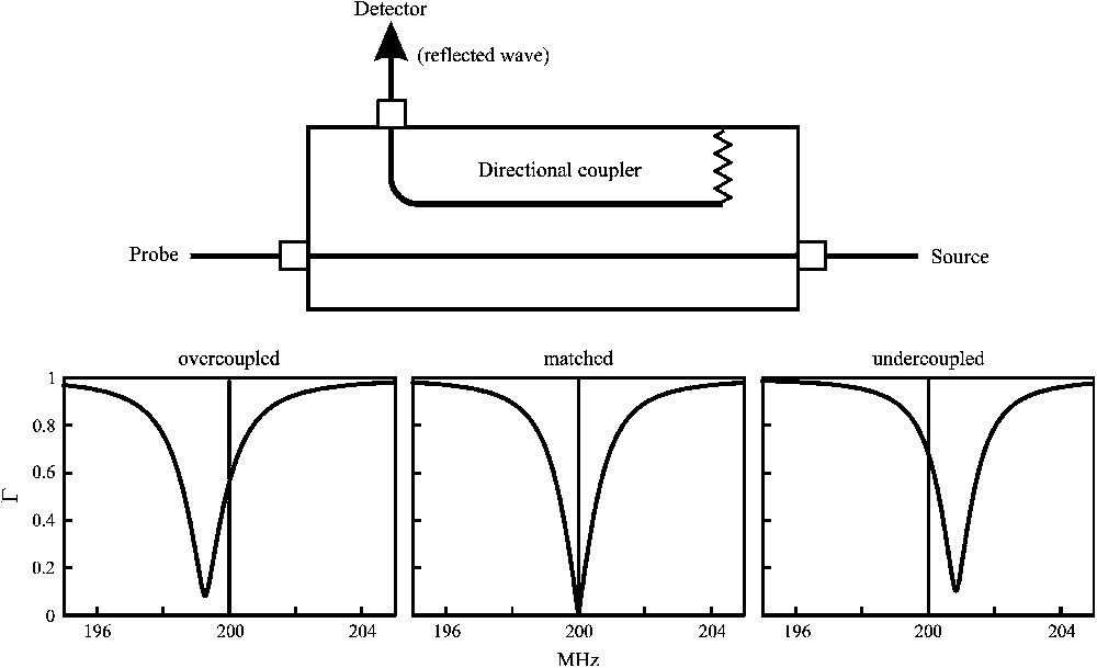
Ratio of reflected to incident RF energy (reflection coefficient Γ) as a function of the frequency when the probe is connected to a given RF power source. Top: experimental set-up. A directional coupler is used to sample the reflected wave at the probe port (the input port as indicated on a conventional coupler). The voltage appearing on the coupled port is proportional to the amplitude of the wave traveling from its input port (connected to the probe) to the output port (connected to the source), which is nothing else than the wave reflected by the probe. When the probe impedance is equal to 50 Ω (the characteristic impedance of the line of the coupler), the reflected wave is null. The detector output is zero. When the probe port is open (high impedance) or shorted, the reflected wave amplitude, and consequently the detector output voltage, has its maximum value.
Bottom: typical displays obtained (“wobble” command on most NMR spectrometers) with different coupling conditions, when the source frequency is spanned over a given frequency range. When the frequency is far away from resonance, all the incident energy is reflected back toward the source (Γ = 1). When the frequency is close to resonance, Γ diminishes until Γ = 0 if the probe is perfectly matched to the spectrometer characteristic impedance (resistive 50 Ω). In this case (center), all the incident energy is absorbed by the probe (coil plus sample). If the probe is not perfectly matched, a fraction of energy is reflected back (overcoupled and undercoupled cases, left and right). The shift in resonance frequency is due to the coupling components (capacitive coupling in the present example).
At this stage, the simulation of the electrical properties of the probe circuit is useful for the following goals:
- - determining all the resonant modes of the probe, and
- - featuring all the probe components and parameters (capacitors, inductors, coupling coefficients) necessary to tune and match the circuit at the frequency of interest, for any resonant mode.
Then, the spatial distribution of the so-called rotating frame components B1+ and B1− of the RF magnetic field can be estimated for any resonant mode, using the following equations [2,12,13]:
| (1) |
In these equations, u and v refer to the complex components of the total magnetic field, which is the sum of all the magnetic fields created by the complex current (Iuk + iIvk) flowing in conductor k. For example, Bux is the total RF field component, along the x axis of the laboratory frame, created by all the currents that are “in-phase” with a given reference which can be chosen as one of the exciting RF sources. Bvx is the same component, but created by all the currents that are “90° out-of-phase” with the reference. The complex components of the current in each conductor are obtained from the linear circuit simulation of the probe electrical network. The relative phase of the currents in every conductive elements is of great importance in predicting the detailed field components relevant to the MR experiment [13].
The x and y components in the rotating frame can be viewed as the components of a complex valued field [2]:
| (2) |
| (3) |
The field components in the laboratory frame, required in Eq. (1), are derived assuming the quasi-static approximation and using the use of the Biot–Savart's law [15]. Also, the probe is assumed to be empty (without sample). Despite these approximations, a large number of basic properties of the probe can be accurately described and understood.
A quantitative evaluation of the magnetic field homogeneity is finally given by a histogram of the magnetic field amplitude within a given ROI (Region Of Interest) [16].
The simulation permits the optimization of the probe geometry in order to get the desired spatial field distribution, to achieve its construction in practice and to evaluate its quality by a comparison of the predicted performances with those measured by means of real experiments.
The decisive criterion will be the probe sensitivity, given by Refs. [3,17,18]:
| (4) |
4 Axial resonators
The symmetry properties of a volume resonator are governed by the direction of the current flow on the surface of the probe conductors (due to the skin effect; at frequencies larger than a few MHz, the RF currents are confined in a very thin region close to the conductor surface).
The magnetic field being perpendicular to the current direction, one can define two kinds of resonators, those creating a magnetic field along their symmetry axis (axial resonators) and those creating a magnetic field perpendicular to their symmetry axis (transverse resonators).
Fig. 3 represents the two current distributions that create a perfectly homogeneous field, polarized along the resonator axis (axial resonators).
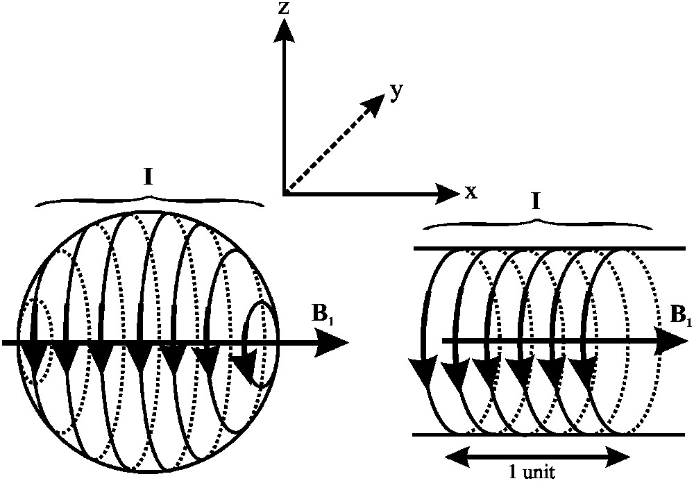
Ideal axial resonators. Equal currents are carried in each elementary “filaments”, evenly positioned on the surface of the conductor. This corresponds to a sinusoidal current density on the surface of the sphere and a constant current density on the surface of the cylinder. Ideally, the cylinder is assumed to be infinite in length. The magnetic field is oriented parallel to the symmetry axis of the coil.
For accessibility reasons, the ideal spherical geometry cannot be realized. In practice, it is approximated by two or four coils, as, respectively, in the Helmholtz and the Hoult–Deslauriers (HD [21]) designs. In either design, each isolated coil is tuned to a given resonant frequency using a capacitor in such a way that, when coupled, the whole system exhibits a resonant mode at the required frequency. The current is evenly distributed in the Helmholtz coils and the RF field homogeneity is maximum when the distance between the two coils is equal to their diameter. In the HD design, both the geometry and the current distribution must be optimized for the field homogeneity. The required current distribution is obtained from the adjustments of the resonance frequency of each constitutive resonator. Other four-coil configurations have also been recently proposed [22]. They differ slightly from the HD design by the fact that all coils are tuned to the same resonant frequency, making the adjustment simpler. This results also in a slightly different geometry than the HD design.
The ideal cylindrical geometry is a cylinder of infinite length. In practice, the best known approximation of this configuration is the solenoid coil. This coil gives the best sensitivity of magnetic resonance among all resonator designs. It is therefore the preferred choice whenever possible, but at relatively low frequencies. Solid- state NMR makes use of this kind of resonator. It is also used as micro-coils [23] to build high-sensitivity NMR probes for very small quantities of biological samples [24]. It exhibits, however, an inherent heterogeneity in a plane perpendicular to its axis due to the helical winding (Fig. 4). It becomes also self-resonant at a relatively low fd product. The self-resonance is expected to occur when the coil impedance approaches 600 Ω, corresponding to fd of the order of 4–5 MHz m for a well designed solenoid coil.

Mapping of the rotating component of the B1 field in the xy, yz and xz planes, for a solenoid coil having 5 turns (upper), 50 turns (middle) and a loop–gap (lower). The photos to the left represent a solenoid with 8 turns (upper) and a small loop–gap resonator (lower) made of a thin copper foil (0.25 × 12 × 37 mm) wound on a PTFE former (diameter 12 mm) enclosing a sample tube (8 mm). The mapping have been simulated from the calculation of the magnetic field components for each design. This is represented as an image that would be obtained after a 4pw–pw pulse sequence [25] where pw is set equal to the 90° pulse length at the center of the coil. The first 4pw pulse sets up the longitudinal magnetization as a function of the B1 amplitude. The second pulse (pw) reads out the amplitude of the longitudinal magnetization resulting from the preceding period. Due to the choice of pw, the magnetization is left unchanged by the first pulse at the center of the coil. (For visualizing the color information in this figure, the reader is referred to the web version of this article.)
The loop–gap [1], a one-turn solenoid coil (Fig. 4), provides a convenient solution for solving both problems. This ultra-high frequency (UHF) resonator has the same structure as the magnetron resonant cavity, conceived during the 1940s. It has been proposed as a low-frequency EPR resonator in 1969 [8a,b] and later [9], and was proposed as an NMR probe in 1981 [26]. Its sensitivity is expected to be that of a solenoid. Indeed, it can be demonstrated theoretically that the sensitivity of a solenoid coil is almost independent of the number of turns [12].
The magnetic field's homogeneity is improved (Fig. 4), as compared to that of the solenoid, in a plane perpendicular to the symmetry axis, due to the removal of the helical winding. It is also improved in the axial direction, due to the increase of the current density on the edges of the conductive sheet.
4.1 Current distribution
A general property of flat conductors driven by a current is that the current density increases near the foil edges that are parallel to the current flow (Fig. 5) [27]. It should be noted at this point that the current density results from an inductive effect which should not be confused with the skin effect. This current distribution appears at low frequencies and becomes frequency independent when the reactive impedance is much larger than the zero frequency (DC) resistance. This occurs at 0 Hz for superconductors and at some kHz for conventional conductors (copper, silver, etc.). At radiofrequencies, well above the 10–100 kHz range, the current density does not change until the wavelength becomes of the same order of magnitude as the conductor dimensions.
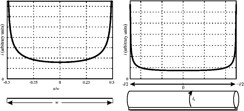
Current density on a flat strip (left) and on the loop–gap surface (right). The current on the strip, assumed infinitely long, is flowing in a direction perpendicular to the paper sheet. The current density increases strongly on the edge of the conductive foil and is relatively uniform near the center. The current distribution fulfils the boundary conditions on the (magnetic) field vector at the surface of the (assumed perfect) conductor [27]. The current on the loop–gap (left) presents a similar distribution. In this case, the current flows on parallel circular filaments on the coil surface from one edge of the gap to the opposed one. The high current density at the extremities of the coil contributes to improve the homogeneity of the magnetic field inside the loop. Such a current distribution is almost independent of the thickness of the conductors and of the frequency (from 0 Hz for superconductors to a few kHz for a copper foil). It should not be confused with the skin effect, which is frequency dependent and which describes the current density inside the conductor.
Quantitatively, the current density can be estimated by different methods. In one method [12], the current density is calculated from the boundary condition that the magnetic field component perpendicular to the conductor surface must be zero everywhere.
For the loop–gap, the current density is described by a discrete set of circular filaments of current {Ik} flowing on a radial path from one edge of the gap to the other (Fig. 6). The boundary condition for the magnetic field is written similarly for a discrete set of positions {j}. This is expressed as:
| (5) |
| (6) |
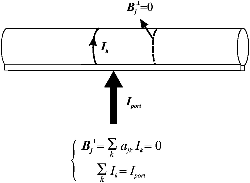
Outline of the current density calculation method [12] applied to the loop–gap. The current density on the conductor is described as a discrete set of regularly spaced circular filaments of current Ik, as shown on the figure. The boundary condition on the magnetic field vector at the surface of the conductor is sampled on a discrete set of positions located between the current filaments (in order to avoid any singularities). The field component perpendicular to the conductor at that point (j) is calculated by adding the contributions ajkIk from all the current Ik. Due to symmetry, the amplitude of this component is independent of the radial position. Hence the number of positions where the magnetic field is sampled is equal to the number of current filaments minus one. In practice, this number may range from 10 to 1000 (or more without any difficulty) depending on the desired resolution of the current distribution. All the boundary conditions at locations j are written as a set of linear equations with Ik as unknowns, A{Ik} = b. At this point the linear system of equations is incomplete (all elements of the b vector are null). Adding the condition that the sum of all current filaments must be equal to the total current carried by the conductor (Iport), one obtains a solvable system of equations for Ik. The matrix elements ajk depend only on the geometry of the problem. A similar approach can be used to calculate the current distribution on flat or on cylindrical conductors where the current flows along the longitudinal direction. Such a method has been used for calculating the current distribution on the shield surrounding a given coil.
Another method, providing identical results, is based on the partial inductance concept [29]. This approach developed during the beginning of the past century for inductance calculations is nowadays essentially used in the microelectronic industry [30,31]. Briefly, the method consists in the decomposition of each conductor into smaller segments forming a linear network of coupled RL (resistance–inductance) components (including possibly a capacitor C). The self- and mutual- partial inductances Lij constituting the network can be calculated by formulae found in the literature [32]. The circuit equations describing the network are solved for the currents and voltages in each RL(C) elements, using a SPICE like simulator [10,11] or any, simpler, linear circuit simulator. In addition to the currents, one can get also the total inductance of the probe. This approach is similar to that implemented in Fasthenry [33] for computing the inductance matrix of a complex network of wire connections. This software can be efficiently used for many MR probe designs.
The partial inductance method has the advantage that it is more general than the previous one, but it is much more demanding as far as computer resources are concerned. As the volume resonators used in magnetic resonance exhibit generally high symmetry, the first method (direct method) can be used in many cases without too much lack of generality. All the currents' densities calculated here were performed using the direct method.
5 Transverse resonators
A cosine-dependent distribution of linear currents flowing parallel to a cylindrical axis produces also a homogeneous magnetic field inside the cylinder [14] (Fig. 7). The magnetic field is oriented perpendicular to the cylinder axis. The resonators built according to this configuration have a very good sample access, especially when used inside a superconductor magnet.
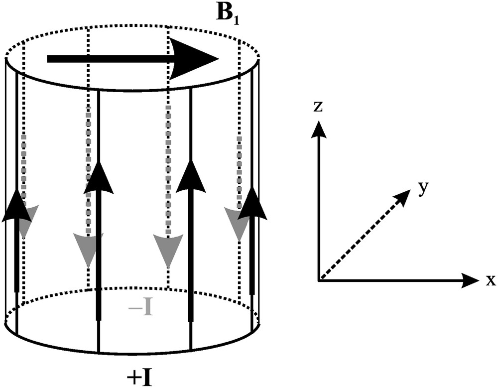
Ideal transverse resonators. The current on the surface of the front-half of the cylinder is out-of-phase with the current on the back-half of the cylinder. The current amplitude has a cosine dependence on the azimuth angle. Ideally, the cylinder is assumed to be infinite in length. The magnetic field is oriented perpendicular to the symmetry axis of the coil.
In a similar way as the Helmholtz coil, the crudest approximation of the cylindrical cosine current distribution is the widely used “saddle coil” (Fig. 8). It is constituted of two rectangular coils, either connected in series (the most frequent stable configuration) or coupled together like in the Helmholtz free-element resonator. The optimum homogeneity is obtained when the angle subtended by each coil is equal to 120°.

B1 mapping in the xy plane (middle), using the 4pw–pw pulse sequence (see legend of Fig. 4), of the optimized saddle coil (top) and slotted tube (bottom). The histograms of B1+/I amplitudes (right) are calculated in a cylinder having a diameter equal to 90% of the coil diameter. The RF field homogeneity of the slotted tube is clearly better than that of the saddle coil. The improvement is at the expense of a slight decrease of the RF field amplitude. I is the total current that flows on each half cylindrical surface of the coil. (For visualizing the color information in this figure, the reader is referred to the web version of this article.)
UHF versions of such a resonator have been developed during the 1970s as a transmission line resonator [34] and subsequently as the slotted tube (ST, [4]), and the slotted cylinder (SC, [5]), also known as the Alderman–Grant resonator (AGR, [6]). All these resonators are based on a common structure constituted of two conductive sheets shaped on a cylinder and driven by current in opposed phase (Fig. 8). The homogeneity of the magnetic field created by this structure is optimum when the angle subtended by the conductive sheet is near 90°. It is also slightly improved as compared to the saddle coil. The current density is here expected to increase near the conductor edges parallel to the cylinder axis, which is also the direction of the current flow. This is visible on the magnetic field map shown in Fig. 8.
5.1 Toward the cosine current distribution
There are mainly two designs that attempted to mimic the ideal current cosine distribution around the cylinder. One is the “birdcage” [13,35], which is nowadays the widely used MRI configuration. It is basically constituted of identical resonators connected together and evenly distributed around the cylinder (Fig. 9). The relative phases and amplitude of the currents flowing in the legs depend on the resonant modes. This is shown in Fig. 10 for a 12-leg birdcage that has 6 resonant modes. It can be seen that the required cosine distribution around the cylinder is obtained only with the first mode. The corresponding magnetic field is indeed homogeneous inside the coil volume. For this mode, the magnetic field homogeneity improves further as the number of elements increases. In practice, the number of legs is limited to 12–16, possibly 32 for large resonators at low frequency, which is a compromise between a good homogeneity and manufacturing difficulties. An exception is the Varian Milliped™ resonator [37] which includes about 1000 legs tuned by distributed capacitances around the cylinder.
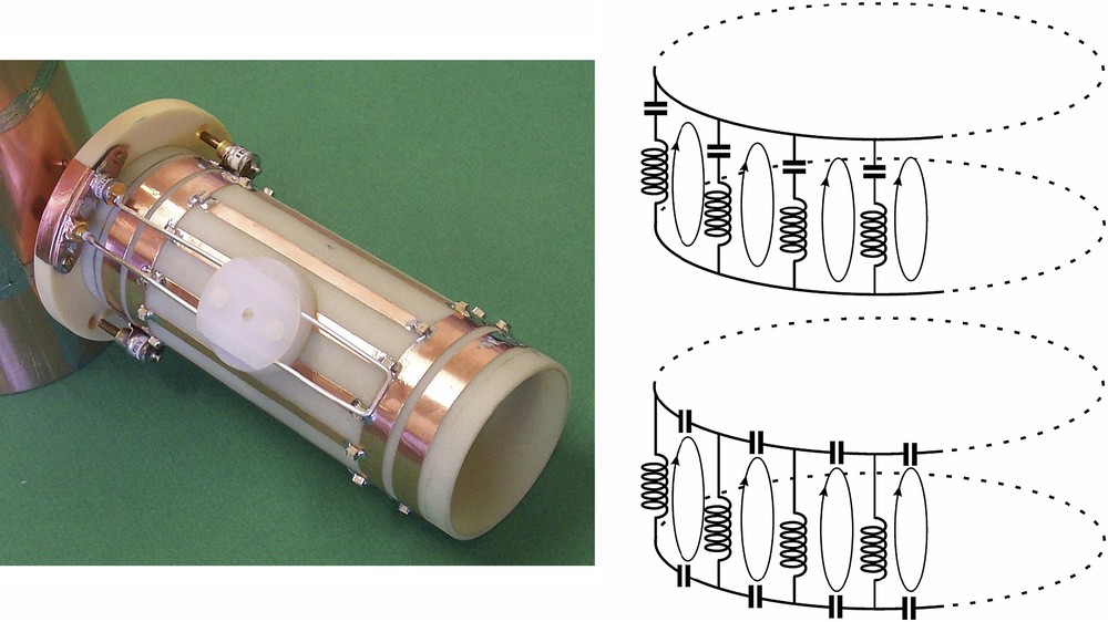
Left: photo of a 200-MHz birdcage resonator designed for small-animal MRI. The inductive coupling is made through a loop running parallel to the coil legs. The birdcage is of the low-pass type, each leg being tuned by two capacitors located at their ends. The two additional rings, coaxial to the birdcage end rings, are the tuning “link” rings [36].
Right: simplified electrical circuit of the low-pass (upper) and high-pass (lower) birdcage coil.
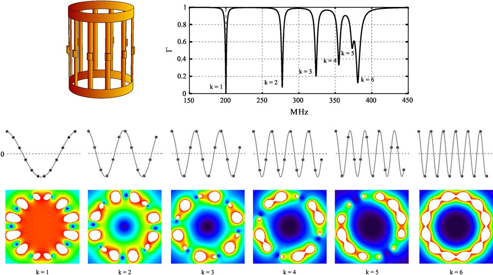
The 6 resonant modes of a 12-leg birdcage coil (top) are shown by the reflection coefficient Γ as a function of frequency. The spectrum represented here has been simulated using “simprobe” [12]. The current amplitude in each leg is represented (middle) by dark dots as a function of the leg number, for each resonant mode. The corresponding B1+ RF field amplitude is shown at the bottom. The first k = 1 mode has the required cosine current distribution as a function of the azimuth angle. It is therefore the sole mode leading to a homogeneous B1 field distribution (bottom). All other modes produce RF field gradients characterized by a null (dark) at the center of the coil. (For visualizing the color information in this figure, the reader is referred to the web version of this article.)
In the birdcage resonator, the cosine current distribution is obtained naturally for one of its resonant mode, but it is quite sensitive to the geometry and component values. In order to implement a robust design, an attempt to force the cosine current distribution has been made by connecting, in parallel, a number of wires judiciously positioned around the cylinder [38]. This assumes that the current is evenly distributed in the wires. In practice, this cannot be the case due to the mutual inductance between the legs. The current distribution depends on the ratio of self- to mutual inductances. If the legs wire is very thin, the self-inductance is much larger than the mutual inductance with the other legs and the current distribution is close to the ideal cosine distribution. But for obvious reason of sensitivity, the wire cannot be made as thin as it should be. On the contrary, if the wires are made of large strips, covering almost all the surface of the cylinder, the self-inductance is much smaller and the current distribution tends to that of the slotted tube. This so-called cosine or Bolinger coil [38] has, however, the simplicity of the slotted tube, whereas the magnetic field homogeneity is still slightly improved.
6 Shielding effects
The signal to be detected in MR experiments being usually very small, it is preferable to shield the probe in order to reduce the interactions of the coil with the environment. This prevents the receiver from spurious signals and protects also the surrounding electronics from intense radiofrequency perturbations due to the high-power pulses. Furthermore, the shield limits the radiation losses that may occur at relatively high frequencies. It diminishes also the capacitive coupling (Faraday shield) with the enclosing metallic parts, which is responsible for the occurrence of parasitic common mode currents.
Usually the shield is a conductive cylinder placed around the probe. This has some consequences on the resonator behavior. First of all, the resonant frequencies generally increase due to the decrease of the probe inductance. Secondly, and probably less often considered, the magnetic field inside the resonator (in the sample volume) decreases when the ratio of shield to resonator diameters becomes smaller. This is shown in Fig. 11 for a shielded saddle coil.
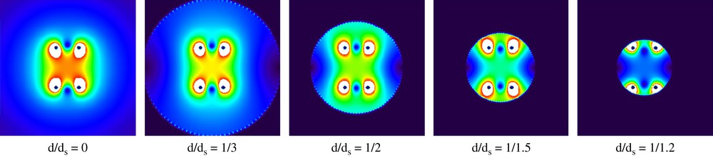
Shielding effect on the RF field distribution of a saddle coil. The field map is calculated from the current distribution estimated using the “direct method” outlined in the text. Note the decrease of the magnetic field amplitude inside the coil as the shield diameter decreases (from left to right). In contrast, the field amplitude increases between the coil conductors and the shield. This is a general effect. It has been already described for axial (for example, [9]) and transverse resonators (for example, [12, 41,42]). (For visualizing the color information in this figure, the reader is referred to the web version of this article.)
All these effects can be easily understood using the images theory [15,39,40,41,42]. Each current line of the resonator inside the cylindrical shield creates a mirrored image represented by a current line of opposed phase, located outside the shield cylinder at a position ri given by [39]:
| (7) |
The shield may have some dramatic consequences on the probe sensitivity, especially when the losses arise essentially from the sample. In this case, the B1/I ratio (see below) is decreasing, while the resistance of the loaded probe will not change at all.
7 What is expected from a given probe?
The probe sensitivity is of great importance in MR experiments due to the inherently very low macroscopic magnetization that should be detected. Eq. (4) indicates that the sensitivity depends mainly on two factors: the ability of the probe to convert a given current I into a magnetic field, which is represented by the term (B1/I) and its ability to create a given current I from a supplied RF power P, represented by (1/√r).
The first factor depends entirely on the resonator geometry. The second factor depends on a large number of parameters that must be optimized for each particular design. For example, a cryo-probe, in which the resistance of the conductors is extremely small, improves significantly the sensitivity, which strongly depends on the working frequency, on the “filling factor” and on the conductive properties of the sample [18].
The optimization of the probe resistance is outside the scope of this short review. We will discuss rather the comparison of the “magnetic efficiency” (B1/I) among the different kinds of homogeneous resonators so far described.
The main difficulty in comparing the magnetic efficiencies of all the resonators (Table 1) is to correctly define the current I value that enters the ratio B1/I. This is given by the current of the ideal configurations (Figs. 3 and 7). For example, the current I for the Helmholtz coils is twice the current that flows in each coil. Similarly, for the saddle coil, the current I is half the current supplied to the coil. In contrast, I is equal to the supplied current for the slotted tube. For axial resonators (solenoid, loop–gap, Helmholtz coils or Hoult–Deslauriers four-coil resonator [21]), I is still defined as the total current supplied to the coil.
Rotating frame component of the RF magnetic field (B1+, gauss) at center of the homogeneous resonators
| Ideal axial resonator (sphere) | 4.19 I/d |
| Helmoltz coil | 5.03 I/d |
| Hoult Deslauriers coil | 4.49 I/d |
| Solenoid | 4.44 I/da (6.28/lD) |
| Ideal transverse resonator | 3.14 I/d |
| Saddle coil | 3.46 I/d |
| Slotted tube | 3.39 I/d |
| Birdcage | (3.06–3.14) I/d |
a Note: the value is for a solenoid that has its length equal to its diameter (lD = d√2).
The return path currents are another source of complication for comparing the B1/I efficiency among the transverse resonators. In fact, as Fig. 12 shows, the magnetic field amplitude at the center is maximum when the ratio of the length to the diameter (l/d) is equal to √2. When the ratio is smaller, the magnetic field decreases very quickly and this should be avoided.

Magnetic field amplitude at center of a transverse resonator, taking account of the return path currents. The maximum value is reached when l/d is equal to √2 and is close to the plateau value corresponding to an infinite length coil. For lower l/d values, the magnetic field amplitude decreases dramatically with the length of the coil.
Therefore, B1/I is inversely proportional to the diameter of the coil for all the homogeneous resonators (Table 1). All axial or transverse resonators exhibit almost the same efficiency, with a slight advantage to the axial configuration.
7.1 Some orders of magnitude
It could be useful to have in mind some orders of magnitude for the required current and power that would produce a pulse of desired length. As an example, we will consider a NMR probe including a 5.5-mm proton coil and a 10-mm decoupling X coil. This is a typical arrangement found in any liquid high-resolution NMR spectrometer. The diameter of the proton coil is made slightly higher than the standard 5-mm sample tubes in order to accommodate the coil holder and to allow for the thickness of the wires. These coils may be saddle coils, slotted tubes or AGR, having an almost identical efficiency B1/I. We thus assume that B1 is given by:
| (8) |
Table 2 shows the required current values that should be applied during the excitation pulse, assuming that 90° pulse lengths of 5 μs and 15 μs are desired for proton and carbon (X nucleus), respectively. The current values are quite high, indicating also that the voltage across the capacitor may easily reach the breakdown limit. If this arises the probe is said to be “arcing”, a phenomenon that probably most NMR users have encountered. For solid-state NMR, the required pulse lengths are usually shorter (down to 1 μs or less). As a consequence, the currents, as well as the voltages across the capacitors, must be about an order of magnitude higher.
Current (I) and power (P) required to rotate the spin magnetization by 90° in 5 μs (proton) and 15 μs (carbon) on a 11.7 T (500 MHz) and 21.1 T (900 MHz) NMR spectrometer
| PW90 (μs) | ν1 (kHz) [B1 (G)] | d (mm) | I (A) | L (nH) | Ceq (pF) | P(W) | |
| Proton coil at 500 MHz | 5 | 50 [11.8] | 5.5 | 20 | 9 | 11 | 28 |
| Carbon coil at 125 MHz | 15 | 16.7 [15.7] | 10 | 48 | 20 | 81 | 90 |
| Proton coil at 900 MHz | 5 | 50 [11.8] | 5.5 | 20 | 9 | 3.4 | 50 |
| Carbon coil at 225 MHz | 15 | 16.7 [15.7] | 10 | 48 | 20 | 25 | 160 |
The current is produced by the application of a RF pulse delivered by a power amplifier (transmitter). The required power can be estimated from the following formula [12]:
| (9) |
| (10) |
For a saddle coil, Ceq is equal to 4C0, but for an AGR, Ceq is equal to C0 [12]. This apparent contradiction results from the fact that the wires of the saddle coil are connected in series, whereas each conductive sheets of the slotted tube can be considered as two wires connected in parallel. Hence, the inductance of a well-constructed saddle coil should be about 4 times the inductance of a slotted tube of the same dimensions. As an example, the inductance of a saddle coil having a diameter of 5.5 mm, a length of 15 mm and wound with a 2-mm wide copper foil is estimated to be 41 nH. This is very close to 4 times the inductance of a slotted tube of the same dimensions, which is estimated to be 9 nH [12] plus the inductance of the connections linking the 2 opposed sheets of the coil. The inductance of the 10-mm carbon coil, assumed to be a slotted tube of 30 mm in length is estimated to be 20 nH.
The corresponding Ceq and power P required to get the current quoted above are given in Table 2. The Q factor is assumed to be 200, which is an average value generally observed for such probes. If required, it can be measured before using Eq. (9).
The required power estimated here compares well with the characteristics of the power amplifiers usually proposed by the manufacturers of spectrometers. In particular, the required power is much greater for the X nuclei than for proton, even if the corresponding 90° pulse length is larger. It should be also noted that P increases with the main magnetic field, B0.
Because the required power is proportional to the square of the desired B1, to get a 1-μs proton pulse length, instead of a 5-μs one, requires a transmitter power 25 times higher. Accordingly, the power amplifiers for solid-state NMR must deliver power levels up to the kW range.
As suggested by the simple considerations developed here, the probe sensitivity depends mainly on its geometry (diameter). The accuracy of the calculations provided by the simple Eqs. (8) and (9) is limited. However, this accuracy is generally sufficient to estimate what could be expected for a given probe geometry in order to optimize any desired experiments.
If a greater accuracy is required, the probe's electrical and magnetic properties can be simulated using more elaborate software, ranging from simple to use and cheap utilities such as “simprobe” [12] to very expensive accurate full-wave electromagnetic simulators. The latter are mainly developed for companies concerned with radio communications (mobiles, WiFi, etc.) and microelectronics, but can be used, maybe after some adaptations, for the simulation of MR probes [3].
In any case, it would be of interest to evaluate the performances of a given probe by measuring the 90° pulse length at a known power level and to compare the results with the predicted ones (as well as with those provided by the manufacturer). This is the method of choice to help in debugging a probe with substandard performances.
8 Leaving the quasi-static conditions
Until now, the quasi-static approximation has been assumed. Increase in the resonant frequency has, however, consequences that will be shortly addressed in this section, essentially for introducing the reader toward the most recent technology. Again, the background that may be acquired with the previous considerations will help in understanding the new developments implied by the increase of the magnetic field used for NMR spectroscopy (up to 20–24 T) and clinical imaging (up to 7 T). At this point, it should be mentioned that mainly proton NMR is an issue. NMR of nuclei of low gyromagnetic ratio is obviously less demanding, as the corresponding frequencies are much lower than for proton. Also, low-field EPR (down to the GHz range) is of concern.
There are, at least, two problems to be considered.
The first problem is related to the coil and sample dimensions relative to the wavelength. This problem is aggravated by a reduction of the wavelength in the coil and in the sample relative to the free-space wavelength. For example, the phenomenon of wavelength compression has been assigned as the major origin for RF inhomogeneity in solenoid coils [43]. On the other hand, the wavelength in a solvent (the sample) is reduced by a factor proportional to the square root of the relative dielectric constant (ɛr). For example, the wavelength in water (ɛr = 78) is only 3.4 cm at 1 GHz, instead of 30 cm in free space.
To outcome the alterations of electromagnetic fields' distribution when the coil dimensions are no longer much smaller than the wavelength, some solutions which have been proposed are shortly described in the following.
- - Segmentation of the coil: when the conductor length is greater than roughly λ/8, it is recommended that the wire is evenly divided with a series tuning capacitor (see for example Ref. [14]). This cancels propagation effects and thereby ensures negligible variation of current amplitude along the conductor. In addition, the resulting distributed capacitance along the conductor greatly reduces conservative electric fields and therefore dielectric losses in the sample [44].
- - Choosing the UHF versions of the basic resonator: for example, replacing the saddle coil with the slotted tube [4–6] or replacing the solenoid with the scroll-coil [7,45], and possibly with the loop–gap [1,8,9,46].
- - Using the transmission line technology: for example, the basic birdcage coil can be replaced with the so-called TEM resonator [47,48]. In these resonators, the basic resonant loops of the birdcage (Fig. 9) are replaced with a set of resonators constituted of inductively coupled transmission lines. These lines are constituted of the conductor and its distributed capacitance with the shield which becomes now an integral part of the probe [49]. Possibly, lumped capacitors are added at the ends of the conductor and soldered to the shield. Higher resonant frequencies can be obtained using the strip line technology that finds more and more applications in the development of a variety of new MR probes (see for example Ref. [50]).
The second problem is related to the alteration of the distribution of the electromagnetic fields by the magnetic and dielectric properties of the sample (central brightening [51]). This phenomenon becomes particularly important for imaging of large samples at high-field (human head at 7 T or human body at 3 T). The development of parallel excitation [52–54] is one of the solutions to solve this problem. Using a set of “independent” coils and adjusting the amplitude and the phase of the current in each coil, it becomes possible to get the desired magnetic field profile in the sample (B1 shimming [55,56]). This new technology is still based on some of the basic coil configurations [57] described so far. But a number of designs use the simplest component, which is a simple loop of wire (the so-called surface coil). This coil creates a heterogeneous distribution of magnetic field in its vicinity. The whole probe is a combination of a number (from 2 to 128 or more) of magnetically decoupled surface coils in an “array” [58]. With such an array, it is possible to obtain a homogeneous signal excitation and/or response in a large volume, still close to the surface of the array. This approach is the basis of the so-called SENSE imaging, for receiving [59] and for transmitting [60]. These new concepts, combined with the coil technology outlined in the preceding paragraph [61–64], are nowadays pushing the limits of high-field imaging of large samples.
It is also worth to mention that EPR imaging of whole mice (a large lossy biological sample) at very-high frequency (1.2 GHz) has been recently reported to be feasible using a single loop multi-gap resonator [65], a configuration which is close to the basic loop–gap resonator.
9 Conclusions
In the present review we have attempted to describe only the very basic properties of various homogenous resonators in order to provide some help for choosing a particular design, taking into account the specific characteristics of the planned experiments. We hope to have shown that using simple formulae it is indeed possible to make some initial evaluation leading to a particular design which can subsequently be optimized using more elaborate tools, also briefly presented here.
A “universal” probe design that fits with all kinds of experiments does not exist. The choice should be made on a number of experimental conditions which could be considered in the following order.
It will depend firstly on the geometry of the experiment:
- - what is the magnet geometry and the required sample accessibility (axial or transversal resonator)?
- - what is the sample volume and the frequency of interest (HF or UHF designs)?
- - what is the magnet bore diameter (determining the shield geometry, hence the magnetic efficiency of the resonator)?
The next choice may be with respect to the RF magnetic field homogeneity. If this is the most important criterion, the choice is evidently the birdcage. But, the ease of construction may be another criterion, especially when a multiple tuned probe is required. In this case, a cosine coil [38] or a slotted tube [4–6] may be preferred.
Between all types of homogeneous resonators having almost the same B1/I efficiency, the final optimization of a design will be dictated by the probe efficiency in converting a given power P into a given current I, at the desired working frequency. This consists essentially in minimizing the resistive losses of the probe conductors and the electric field within the sample. This point has been already addressed in other reviews (see for example Refs. [3,18]).
10 Note added in proofs
The current density on the loop-gap (or hollow cylinder) has been already calculated by a method similar to the "direct method" presented here, with identical results (A. Labiche, S. Kan, A. Leroy-Willig and C. Wary, Rev. Sci. Instrum. 70 (1999) 2113).
Acknowledgments
One of the authors (M.L.) thanks the Institut Curie and the Cancéropole Île-de-France for financial support. The 2D maps have been drawn using the “plot_field” software [12] which is built on the DISLIN library [66]. The author of this library (Helmut Michels) is acknowledged for allowing the scientific community to use his work, free of charge. Jean-Claude Beloeil (CNRS, Orléans) and Brigitte Gillet (CNRS, Gif-sur-Yvette) are acknowledged for their support in our probe developments.