Droplets and jets in microfluidic devices

Pierre Guillot; Armand Ajdari; Julie Goyon; Mathieu Joanicot; Annie Colin

doi:10.1016/j.crci.2008.07.005

Droplets and jets in microfluidic devices

Pierre Guillot ¹ ; Armand Ajdari ² ; Julie Goyon ¹ ; Mathieu Joanicot ¹ ; Annie Colin ¹

¹ Rhodia Laboratoire du Futur, Unité mixte Rhodia-CNRS, Université Bordeaux I, UMR 5258, 178, avenue du Docteur Schweitzer, 33608 Pessac, France
² Laboratoire de Physico-Chimie Théorique, UMR CNRS-ESPCI 7083, 10, rue Vauquelin, 75231 Paris cedex 05, France

Comptes Rendus. Chimie, Volume 12 (2009) no. 1-2, pp. 247-257.

Résumés

Anglais
Français

When immiscible fluids flow in microchannels, monodisperse droplets or jet are obtained depending upon the flow rate of the aqueous phase and the oil phase. In this work, we present experimental data showing that the confinement and the shape of the geometry play a fundamental role. We analyze the stability of the jet in the framework of the lubrication at low Reynolds number. In cylindrical geometry, we relate the transition between the droplets regime and the jet regime to the absolute/convective transition of the Rayleigh Plateau instability and reach a remarkable agreement with the data. In rectangular geometry, we follow the same analysis and point out the existence of an absolutely stable bidimensional jet.

Lorsque des fluides non-miscibles coulent dans des microcanaux, des gouttes monodisperses ou des jets sont produits selon les débits de fluides injectés. Dans ce travail, nous présentons des résultats expérimentaux montrant que le confinement et la forme des canaux jouent un rle fondamental. Nous analysons la stabilité de l'coulement dans le cadre de l'approximation de la lubrification à faible nombre de Reynolds. En géométrie cylindrique, nous relions la transition entre le régime de goutte et le régime de jet à la nature de l'instabilité de Rayleigh Plateau (absolue ou convectée). En géométrie rectangulaire, nous mettons en évidence l'existence de jet bidimensionnel absolument stable.

Métadonnées

Reçu le : 2008-03-26
Accepté le : 2008-07-16
Publié le : 2008-11-17

DOI : 10.1016/j.crci.2008.07.005

Keywords: Instabilité Convecteé, Jets, gouttes, microfluidique
Mots clés : Instabilité Convecteé, Jets, gouttes, microfluidique

Affiliations des auteurs :

Pierre Guillot ¹ ; Armand Ajdari ² ; Julie Goyon ¹ ; Mathieu Joanicot ¹ ; Annie Colin ¹

@article{CRCHIM_2009__12_1-2_247_0,
     author = {Pierre Guillot and Armand Ajdari and Julie Goyon and Mathieu Joanicot and Annie Colin},
     title = {Droplets and jets in microfluidic devices},
     journal = {Comptes Rendus. Chimie},
     pages = {247--257},
     publisher = {Elsevier},
     volume = {12},
     number = {1-2},
     year = {2009},
     doi = {10.1016/j.crci.2008.07.005},
     language = {en},
}

TY  - JOUR
AU  - Pierre Guillot
AU  - Armand Ajdari
AU  - Julie Goyon
AU  - Mathieu Joanicot
AU  - Annie Colin
TI  - Droplets and jets in microfluidic devices
JO  - Comptes Rendus. Chimie
PY  - 2009
SP  - 247
EP  - 257
VL  - 12
IS  - 1-2
PB  - Elsevier
DO  - 10.1016/j.crci.2008.07.005
LA  - en
ID  - CRCHIM_2009__12_1-2_247_0
ER  -

%0 Journal Article
%A Pierre Guillot
%A Armand Ajdari
%A Julie Goyon
%A Mathieu Joanicot
%A Annie Colin
%T Droplets and jets in microfluidic devices
%J Comptes Rendus. Chimie
%D 2009
%P 247-257
%V 12
%N 1-2
%I Elsevier
%R 10.1016/j.crci.2008.07.005
%G en
%F CRCHIM_2009__12_1-2_247_0

Pierre Guillot; Armand Ajdari; Julie Goyon; Mathieu Joanicot; Annie Colin. Droplets and jets in microfluidic devices. Comptes Rendus. Chimie, Volume 12 (2009) no. 1-2, pp. 247-257. doi : 10.1016/j.crci.2008.07.005. https://comptes-rendus.academie-sciences.fr/chimie/articles/10.1016/j.crci.2008.07.005/

Version originale du texte intégral

1 Introduction

Emulsions, foams, dispersions are example of multiphase fluids. These materials are ubiquitous in nature and in industry: e.g., concentrated emulsions, colloidal dispersion, granular flows, in the food and in the cosmetic industry [1]. In many of these applications the dispersion is polydisperse and poorly controlled due to the difficulties encountered during the emulsification process. Renewed interest in emulsification field has been brought by the demonstration that microfluidic devices may produce highly monodisperse droplet at the micrometer size [2]. This control of the droplet size distribution has been demonstrated to be very useful in new applications and for developing new technologies. Monodisperse capsules, multiple emulsions [3,4] or janus particles [5] have been produced using microfluidic devices. The perfect control of the size and velocity of droplet allows one to provide measurements of interest to the biological and chemical communities. Droplets in microfluidic devices has been used to study chemical reaction kinetics on millisecond time scales [6] by injecting reactive chemicals together to form drops and in developing platform for crystallisation and phase diagram [7–9]. Droplets are particularly advantageous for this sort of study because reagents are not dispersed beyond the boundary of the drop. In this article, we deal with the mechanisms involved in the droplet formation. We first present an overview of the study of droplets formation in microfluidic devices. We then report some experiments in various geometries and we present a simple analytic model allowing us to predict the nature of the flow. Section 3 is devoted to cylindrical geometry. Section 4 deals with rectangular geometries which are commonly encountered in microfluidic devices.

2 Biphasic flow in microfluidic devices

Biphasic flow has been widely studied in microfluidic devices [10]. The wetting properties [11] of the microchannel crucially control the patterns obtained [12]. Direct emulsions are produced in glass devices whereas, an inversed one is produced in PDMS devices. The nature of the flow does also depend upon the geometry of the microchannel. Using a flow focusing geometry, Anna et al. [2] have studied drop formation in liquid–liquid systems as a function of flow rates and flow rate ratios of the two liquids. They present a phase diagram including one regime where drop size is comparable to orifice width and a second regime where drop size is dictated by the diameter of a thin “focused” thread, so drops much smaller than the orifice are formed. They point out that both monodisperse and polydisperse emulsions can be produced. Drops are not the single pattern that may be obtained in microfluidic devices. Jets or truncated jets [13] are commonly encountered for high values of the non-wetting phase flow rate. Surface tension and the viscosity ratio rule the drop size and the transition between the parallel flow regime and the drop regime [14]. The understanding of the droplet formation requires the use of flow stability analysis or of numerical computation [15]. Flow stability analysis has been widely used to apprehend break-up scenario in unbounded flowing systems. Determining the conditions required to get an absolute or a convective instabilty allows one to predict the zone of droplets and jets production. Absolute instability corresponds to disturbances growing and propagating both in the downstream and upstream directions. A continuous jet cannot thus exist and typically, drops are released intermittently either right at the injection nozzle or at a finite distance from it to form a dripping jet. At the opposite, convective instability corresponds to perturbations that propagate downstream while they grow, allowing for a long continuous fluid thread to persist. Several experimental studies support this picture and the link between the absolute/convective transition of the instability to the dripping/jetting transition in the observed spatio-temporal behaviour of the biphasic flow [16–24]. In the following, we will apply these considerations to flows in cylindrical microfluidic devices and in rectangular cross-section microfluidic devices.

3 Drops and jets in microfluidic devices with a circular cross-section

3.1 Experimental results in cylindrical geometries

We generate a jet in a cylindrical glass capillary of inner radius R_c [25], using as a nozzle a glass capillary of square cross-section with a tapered end (see Fig. 1).

Fig. 1
Flow studied. An internal fluid flows with a flow rate Q_i in a an immiscible fluid flowing with a flow rate Q_e. The geometry is a cylindrical one with a radius R_c. The radius of the inner fluid is $r_{i}^{o}$ .

The outer dimension of this square capillary is very close to the inner diameter of the cylindrical tube which ensures good alignment and centering. R_c is in the 200–500 μm range, whereas the radius of the tapered orifice of the square tube is set between 20 and 50 μm using a pipette–puller set up. Syringe pumps are used to inject an inner fluid of viscosity η_i at a rate Q_i in the square capillary and the outer fluid of viscosity η_e at a rate Q_e through the cylindrical capillary. This leads to coaxial injection at the tapered orifice. We observe flow patterns which vary significantly with operational (Q_e, Q_i), geometrical (R_c), and system parameters (η_i, η_e, surface tension). Fig. 2 displays the typical outcome of an experiment where the flow rates are varied for a given system (here the inner solution is 50 in weight glycerine in water solution with η_i 55 mPa s and the outer one a silicone oil for which η_e 235 mPa s). A droplet regime is found for low Q_i, with either droplets emitted periodically right at the nozzle symbol (open circle) or non spherical plug like droplets resulting from the instability of an emerging oscillating jet (filled gray circle). Jets are found in the bottom right corner of Fig. 2 with different visual aspects: wavy jets with features that are convected downstream (open square), and for larger values of Q_i, straight jets (filled square) that persist throughout the cylindrical capillary. For large values of the external flow rate Q_e, we observe what we call jetting: thin and rather straight jets (open diamond) that extend over some distance in the capillary tube before breaking into droplets at a well-defined and reproducible location. This jet length increases with Q_i for a fixed value of Q_e.

Fig. 2
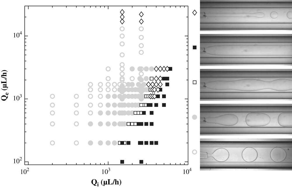
Map of the flow behaviour in the (Q_e, Q_i) plane. The droplet regime comprises droplets smaller than the capillary (○) and plug-like droplets (●) confined by this capillary. Jets are observed in various forms: jets with visible peristaltic modulations convected downstream (□), wide straight jets that are stable throughout the 5 cm long channel (■), and thin jets breaking into droplets at a well defined location (◊). Parameters are R_c = 275 μm, inner viscosity η_i = 55 mPa s, outer viscosity η_e = 235 mPa s, surface tension Γ = 25 mN/m.

3.2 Theoretical description of the droplets jet transition in cylindrical geometries

We now attempt to model these phenomena analytically. To reach this aim, we will perform a linear analysis of the stability of the flow and determine the conditions required to get an absolute or a convective instability. Beyond the importance of viscous forces (the Reynolds numbers are typically small to moderate), the essential contrast with most of the previous studies which focused on unbounded flows is the major role of the microchannel walls which induce parabolic flow profiles and strongly affect the development of perturbations.

In order to get an analytical description, we proceed with approximations. We neglect inertial effects (i.e., as the Reynolds number is small in most of our experiments), and we use lubrication theory (i.e., we formally assume that the wavelengths of the perturbations are long compared to the capillary radius) which has been shown to be remarkably insightful in somewhat related situations [26].

3.3 Lubrication analysis for the cylindrical geometry

We first consider a cylindrically symmetric geometry (see Fig. 1). In a capillary tube of radius R_c are flown two immiscible and incompressible liquids, an “inner” fluid of viscosity η_i is injected at rate Q_i in the stream of an “external” liquid of viscosity η_e flowing at rate Q_e.

In the unperturbed state, the flow is unidirectional with an inner fluid jet of radius $r_{i}^{o}$ and pressure gradients ∂_zP_e and ∂_zP_i in the two fluids that are constants. Together with the boundary conditions at the surface of the jet (continuity of the velocity field and tangential shear stress) and at the walls of the geometry (no slip condition) and local force balance leads to:

Q_{e}^{o} = \frac{R_{c}^{2} r_{i}^{o 2}}{4 η_{e}} (\frac{r_{i}^{o 2}}{R_{c}^{2}} - 1 - 2 \frac{r_{i}^{o 2}}{R_{c}^{2}} \ln (\frac{r_{i}^{o}}{R_{c}})) (\partial_{z} P_{i}^{o} - \partial_{z} P_{e}^{o}) - \frac{π {(R_{c}^{2} - r_{i}^{o 2})}^{2}}{8 η_{e}} \partial_{z} P_{e}^{o}

(1)

and

Q_{i}^{o} = \frac{π r_{i}^{o 4}}{2 η_{e}} \ln (\frac{r_{i}^{o}}{R_{c}}) (\partial_{z} P_{i}^{o} - \partial_{z} P_{e}^{o}) - \frac{π r_{i}^{o 4}}{8 η_{i}} \partial_{z} P_{i}^{o} + \frac{π r_{i}^{o 2} {(r_{i}^{o 2} - R_{c}^{2})}^{2}}{4 η_{e}} \partial_{z} P_{e}^{o} .

(2)

The two pressure gradients are linked through the continuity of the normal stress at the interface:

P_{i}^{o} - P_{e}^{o} = \frac{Γ}{r_{i}^{o}},

(3)

where Γ is the surface tension. For the unperturbed flow, the radius of the inner jet is constant and the two fluids bear the same pressure gradient.

We perform a linear stability analysis and consider the spatial-temporal response of the system to small z-dependent cylindrically symmetric perturbations δQ_e, δQ_i, ∂_zδP_e, ∂_zδP_i and δr_i. We make the perturbations proportional to e^(ikz+ωt) with k and ω complex numbers. As indicated in Section 1, we restrict our analysis to the lubrication approximation, assuming formally that the perturbation wavelength is larger than the capillary radius R_c. In this framework, the expressions obtained for the unperturbed flow can still be used locally, so that the local perturbations in the flow rates read:

δ Q_{e} = \frac{\partial Q_{e}^{o}}{\partial (\partial_{z} P_{e}^{o})} \partial_{z} δ P_{e} + \frac{\partial Q_{e}^{o}}{\partial (\partial_{z} P_{i}^{o})} \partial_{z} δ P_{i} + \frac{\partial Q_{e}^{o}}{\partial r_{i}^{o}} \partial_{z} δ r_{i},

(4)

δ Q_{i} = \frac{\partial Q_{i}^{o}}{\partial (\partial_{z} P_{e}^{o})} \partial_{z} δ P_{e} + \frac{\partial Q_{i}^{o}}{\partial (\partial_{z} P_{i}^{o})} \partial_{z} δ P_{i} + \frac{\partial Q_{i}^{o}}{\partial r_{i}^{o}} \partial_{z} δ r_{i},

(5)

where the partial derivatives are computed using Eqs. (1) and (2).

However, an important difference is that, as the radius of the jet varies, the Laplace law now requires that the two pressure gradients are different:

\partial_{z} (δ P_{i} - δ P_{e}) = - Γ (\partial_{z} (\frac{δ r_{i}}{R_{c}^{2}} + \partial_{z}^{2} δ r_{i})),

(6)

where

δ r_{i} / R_{c}^{2}

is proportional to the curvature in the cross-section of the jet and ∂_z²δr_i to the curvature in the flow direction.

This set of equations is equivalent to computation of the linear response in δr_i, through a second order expansion in powers of $ε = R_{c} / L_{z}$ of the velocity field, where $L_{z} = 2 π / k$ is the characteristic length scale involved in the z direction. We recall that in the lubrication approximation L_z is larger than the capillary radius R_c which implies that ε ≪ 1. Note however, that an additional approximation is required to get these expressions. Specially, in the calculation of the O(ε²) term, where it is equivalent to neglect the pressure gradient created by the zeroth order in ε velocity compared to the one generated by the interface curvature along z. We will quantify more precisely this approximation at the end of this section.

Mass conservation of the incompressible fluids allows to close the system of equations:

δ Q_{e} + δ Q_{i} = 0,

(7)

\partial_{t} (π {(r_{i}^{o} + δ r_{i})}^{2}) = \partial_{z} δ Q_{e} .

(8)

We continue with the following set of dimensionless variables:

x = \frac{r_{i}^{o}}{R_{c}}, λ = \frac{η_{i}}{η_{e}}, \tilde{k} = r_{i}^{o} k, \tilde{ω} = \frac{ω 16 η_{e} R_{c}}{Γ},

\tilde{δ Q_{i}} = \frac{8 η_{e}}{π R_{c}^{4} \partial_{z} P_{i}^{o}} δ Q_{i}, \partial_{z} \tilde{δ P_{i}} = \frac{\partial_{z} δ P_{i}}{\partial_{z} P_{i}^{o}},

\tilde{δ Q_{e}} = \frac{8 η_{e}}{π R_{c}^{4} \partial_{z} P_{e}^{o}} δ Q_{e} and \partial_{z} \tilde{δ P_{e}} = \frac{\partial_{z} δ P_{e}}{\partial_{z} P_{e}^{o}} .

(9)

Eqs. (4) and (5) become Eqs. (10) and (11).

δ \tilde{Q_{e}} = a (x) \partial_{z} δ \tilde{P_{e}} + b (x) δ x + c (x) (\partial_{z} δ \tilde{P_{i}} - \partial_{z} δ \tilde{P_{e}}),

(10)

δ \tilde{Q_{i}} = d (x) \partial_{z} δ \tilde{P_{e}} + e (x) δ x + f (x) (\partial_{z} δ \tilde{P_{i}} - \partial_{z} δ \tilde{P_{e}}),

(11)

where

a (x) = - {(1 - x^{2})}^{2} d (x) = 2 x^{2} (x^{2} - 1) - λ^{- 1} x^{4},

b (x) = 4 x (1 - x^{2}) e (x) = 8 x^{3} - 4 λ^{- 1} x^{3} - 4 x,

c (x) = 2 x^{4} - 2 x^{2} - 4 x^{4} \ln (x) f (x) = 4 x^{4} \ln (x) - λ^{- 1} x^{4} .

Using Eqs. (6)–(8) we obtain the dispersion equation (Eq. 12).

\tilde{ω} = \frac{- i \tilde{k} \cdot x^{3} Ka E (x) + F (x) ({\tilde{k}}^{2} - {\tilde{k}}^{4})}{D (x)}

(12)

where we have introduced a dimensionless capillary number

Ka = \frac{- \partial_{z} P^{o} R_{c}^{2}}{Γ}

and made use of the shorthand notations:

E (x, λ) = - 4 x + (8 - 4 λ^{- 1}) x^{3} + 4 (λ^{- 1} - 1) x^{5},

F (x, λ) = x^{4} (4 - λ^{- 1} + 4 \ln (x)) + x^{6} (- 8 + 4 λ^{- 1}) + x^{8} (4 - 3 λ^{- 1} - (4 - 4 λ^{- 1}) \ln (x)),

D (x, λ) = x^{9} (1 - λ^{- 1}) - x^{5} .

The first term of the dispersion equation $- i \cdot x^{3} Ka (E (x) / D (x)) \tilde{k}$ summarizes the convection kinematics and the mass conservation; the second term $(F (x) / D (x)) ({\tilde{k}}^{2} - {\tilde{k}}^{4})$ describes the convection effect. E and F are positive functions in cylindrical geometry. Ka is a genuine capillary number as it is the ratio between viscous forces $η_{e} V_{e} R_{c} = - \partial_{z} P^{o} R_{c}^{3}$ and capillary forces ΓR_c. We have however used a notation different from the usual Ca to call the reader's attention to the fact that Ka is a capillary number at the scale of the capillary R_c rather than at the scale of the jet. Obviously in contrast with our approach, studies of unconfined jets focus on capillary numbers defined using either the average jet velocity or the velocity at the surface of the unperturbed jet.

The system is stable if all ω_rs are negative. This is not the case. Indeed, low real k values, corresponding to large wavelengths, are unstable since F(x) is a positive value. Note that the instability comes from the k² term which is related to the curvature in the cross-section of the jet. Decreasing the jet radius size, decreases the interfacial area and energy cost and promotes instability. The term k⁴, related to the curvature in the flow direction, is a stabilizing term since undulations in the flow direction increase the interfacial energy cost. With some ω_r positive, an initially localized perturbation generates a growing distortion.

As the perturbation grows, a leading edge profile is selected by the flow, such that the long-time profile is dominated by the mode K_r corresponding to the largest growth rate w_r and an external velocity for the envelope. This leads to the following characteristics for the selected perturbations [27–29]:

v^{*} = \frac{ω_{r}^{*}}{k_{i}^{*}}, \frac{\partial ω_{r}^{*}}{\partial k_{r}} = 0 and v^{*} = \frac{\partial ω_{r}^{*}}{\partial k_{i}} .

(13)

The system is absolutely unstable if there are solutions such that v^∗ is negative and convectively unstable if all the solutions v^∗ are positive. In the former case, a continuous jet can no longer be formed with perturbations propagating backwards. This leads typically to droplets being released intermittently to form a dripping jet, either right at the injection nozzle or at any further point of the entrance zone where the inner stream adjusts its size to the imposed environment. At the opposite, if all v^∗s are positive, the disturbances which grow in time are simultaneously convected downstream and a continuous jet can persist in the system. Fig. 3 gives a schematic representation of the two cases.

Fig. 3
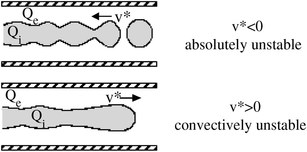
Schematic representation of the absolute instability and the convective instability. The sytem is absolutely instable when one of v^∗ is negative and convectively unstable when all the v^∗ are positive.

Solutions of the dispersion equation that satisfy Eq. (13), lead to four wave vectors that are independent of the imposed flow (or capillary number):

{\tilde{k}}_{1}^{*} = + \sqrt{\frac{9 + 3 \sqrt{7}}{24}} + ⅈ \sqrt{\frac{- 1 + \sqrt{7}}{24}},

{\tilde{k}}_{2}^{*} = - \sqrt{\frac{9 + 3 \sqrt{7}}{24}} + ⅈ \sqrt{\frac{- 1 + \sqrt{7}}{24}},

{\tilde{k}}_{3}^{*} = + \sqrt{\frac{9 + 3 \sqrt{7}}{24}} - ⅈ \sqrt{\frac{- 1 + \sqrt{7}}{24}},

{\tilde{k}}_{4}^{*} = - \sqrt{\frac{9 + 3 \sqrt{7}}{24}} - ⅈ \sqrt{\frac{- 1 + \sqrt{7}}{24}} .

On the other hand, the corresponding dimensionless real part of the growth rate and the dimensionless front velocity,

\tilde{v^{*}} = v^{*} r_{i}^{o} / ω_{o}

, do depend on the capillary number:

ω_{r}^{*} = \frac{Ka E (x) x^{3} \tilde{k_{i}^{*}} + F (x) (5 + \sqrt{7} / 18)}{D (x)} .

(14)

The functions E(x) and F(x) are positive. The wave vectors

k_{1}^{*}

and

k_{2}^{*}

correspond to downstream propagating (and growing) modes with v^∗ always positive. We thus focus on the disturbances associated to

k_{3}^{*}

and

k_{4}^{*}

, which correspond to the same physics as they differ only by a phase factor. The velocity of the associated perturbations is given by:

\tilde{v^{*}} = \frac{Ka E (x, λ) x^{3} - C_{1} F (x, λ)}{D (x)},

(15)

where

C_{1} = (5 + \sqrt{7} / 18) \sqrt{(24 / \sqrt{7} - 1)}

For sufficiently low capillary numbers Ka, the corresponding v^∗ is negative (and ω_r^∗ > 0), whereas in the opposite limit of high flow speeds and large Ka, v^∗ becomes positive. This suggests an absolute to convective instability transition as the flow rate is increased, with the associated transition from dripping to a continuous jet. We thus reach a rather simple analytical prediction for the transition, $\tilde{v^{*}} (Ka, x, λ) = 0$ , plotted on Fig. 4 in the (x, Ka) plane describing operational conditions for various values of the viscosity ratio system λ = η_i/η_e. This plot can be envisioned as a dynamic behaviour diagram with a dripping and a jet regime. For a given λ, increasing the capillary number Ka (i.e., the normalized pressure drop) or the confinement x always eventually lead to a continuous jet. This is physically sound as increasing Ka corresponds to convecting away the perturbations faster, while increasing the confinement x results in slowing down the development rate of the perturbations due to the proximity of the walls. Decreasing λ = η_i/η_e increases the “droplets” regime at the expense of the “jet” regime.

Fig. 4
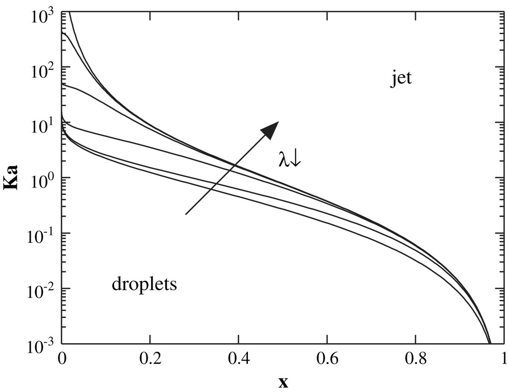
Phase diagram of the instability in the (x, Ka) plane. The lines correspond to various λ equal, from bottom to top, to 10, 1, 0.1, 0.01, 0.001 and 0.0001. Above the lines, the jet is convectively unstable, whereas below the lines the jet is absolutely unstable. Regions below the lines correspond to droplets region.

At this stage, we may comment the validity of our approximations. Two different approximations have been made. First, we used a dispersion equation derived in the lubrication approximation framework. This implies that the parameter $ɛ = r_{i}^{o} / L_{z}$ is smaller than 1. The selected wave vector corresponds to a characteristic length in the z direction, L_z, equals to $L_{z} = 2 π \sqrt{24 / 9 + 3 \sqrt{7}} r_{i}^{o}$ . This leads to a value of $ɛ = r_{i}^{0} / L_{z} = 0.0659 / x$ . Assuming that the use of the dispersion equation obtained in the lubrication approximation framework is valid for ε < 0.2, we can conclude that this hypothesis is valid for x > 0.33. Second, we neglected the recirculations inside the perturbated jets. Indeed, in the calculation of the O(ε²) term, we neglected the pressure gradient created by the zeroth order in ε velocity compared to the one generated by the interface curvature along z. This is valid for x > 0.33 if $η_{i} / η_{e} < 1$ and for x > 0.6 if $η_{i} / η_{e} > 1$ . These ranges of parameters correspond thus to the range where our diagrams are fully valid. Note that this point will prevent us to compare quantitatively our results with the ones obtained in unbounded geometries [22,30].

3.4 Comparison with experiments

We now quantitatively compare our predictions to experimental data obtained for two surface tensions (see Fig. 5) and two capillary radii R_cs (see Fig. 6).

Fig. 5
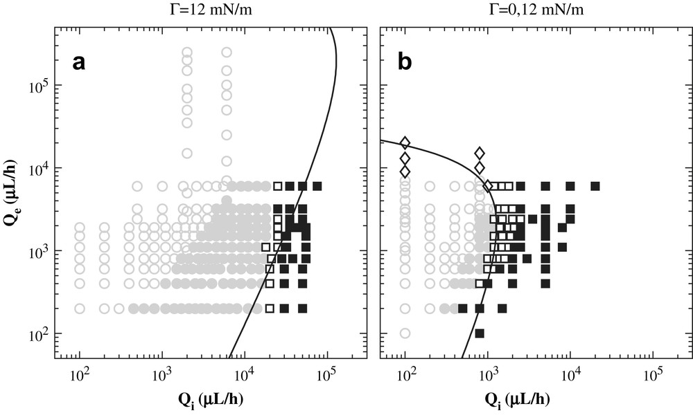
Experimental data (symbols) and theoretical predictions (lines) displaying the effect of a decrease of the surface tension. ○ and ● correspond to droplets □ and ■ to jets. Parameters are R_c = 275 μm, inner viscosity η_i = 1 mPa s, outer viscosity η_e = 3 mPa s. The lines are obtained without adjustable parameters.

Fig. 6
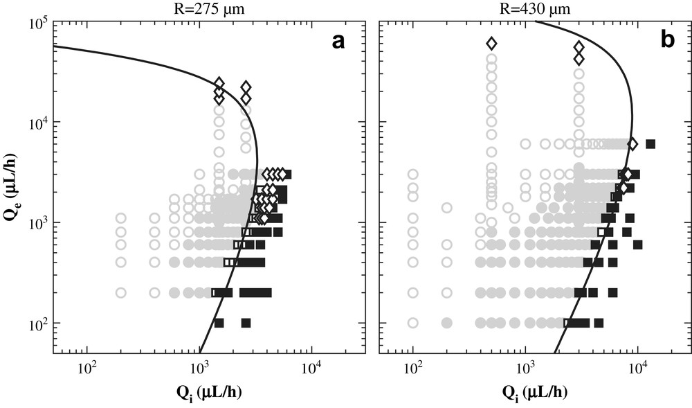
Experimental data (symbols) and theoretical predictions (lines) displaying the effect of an increase of the capillary radius R_c. ○ and ● correspond to droplets, □ and ■ to jets. Parameters are inner viscosity η_i = 55 mPa s, outer viscosity η_e = 235 mPa s, surface tension Γ = 24 mN/m. The lines are obtained without adjustable parameters.

Clearly, given the approximations involved, our simple model describes very well the experimental data with no adjustable parameters, and appears as a powerful predictive tool. A certain level of disagreement is expected for weak confinement (small Q_i large Q_e) as the lubrication approximation is formally invalid in this case. Our model indeed overestimates Ka at the transition for vanishing x, as demonstrated by comparison to the exact result of Gañán-Calvo [30] for unbounded creeping flows. Inertial effects may also slightly alter the picture for the largest outer flow rates. We also report in Figs. 7 and 8 all the experimental data obtained for a given viscosity ratio, but for various surface tensions, various capillary radii, and various flow rates. This shows the relevance of our description in terms of the dimensional variables Ka and x. An additional interest of this mapping onto the (Ka, x) plane of this large set of data is that it collapses relatively well the different types of flows observed within the droplet and jet regimes as can be seen by the grouping of the symbols. In short, droplets correspond to small capillary number Ka and small confinement ratio x, while plugs require larger values of x. At higher values of Ka, increasing the confinement ratio x shifts the behaviour from jetting (with emission of droplets at a large finite distance from the nozzle) to stable jets.

Fig. 7
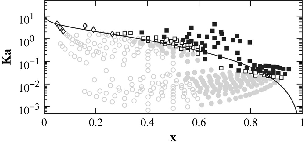
Flow behaviour in the (x, Ka) plane for a given value of the viscosity ratio λ = 0.33. These data correspond to two radii and two surface tensions. The line is the theoretical prediction of our linear analysis for the droplets/jet transition. Symbols are same as in Fig. 2.

Fig. 8
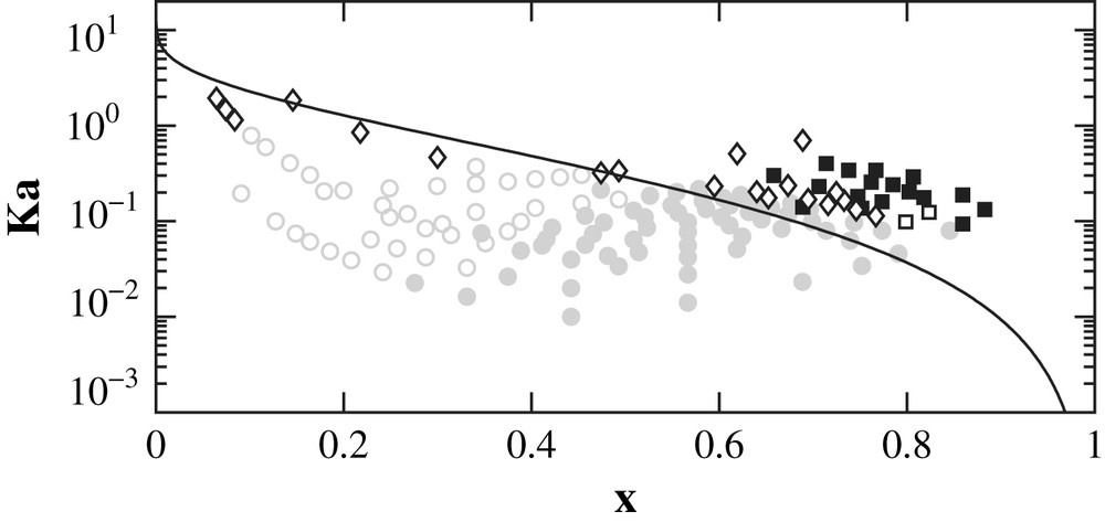
Flow behaviour in the (x, Ka) plane for a given value of the viscosity ratio λ = 4.28. These data correspond to two radii and two surface tensions. The line is the theoretical prediction of our linear analysis for the droplets/jet transition. Symbols are same as in Fig. 2.

4 Drops and jets in microfluidic devices with a rectangular cross-section

4.1 Experiments in rectangular geometries

In this section, we turn to the most commonly encountered geometry in microfluidics, namely that of a microchannel with a rectangular cross-section.

Our microfluidic devices are fabricated using soft lithography technology [31]. Polydimethylsiloxane (PDMS) channels or PDMS–glass channels are used. The microdevices have two inlet arms which meet at a T junction with a funnel design (see Fig. 9). The flow patterns are observed in the outlet channel after the T junction. The inlet channels are connected via tubing to syringes loaded with the fluids. Syringe pumps allow us to control the flow rates of the liquids. In this study the immiscible fluids used are aqueous and oil solutions. Oils are silicone oils (Rhodorsil) of different viscosities and hexadecane (Prolabo). Aqueous solutions are dilute solutions of Sodium dodecyl sulphate (SDS) (Merck) above the critical micellar concentration (cmc) in water (cmc = 0.24 wt%) or in a mixture of glycerine (Prolabo) and water. Adding glycerine allows us to match the optical index of the aqueous solution with silicone oil and thus, enables us to perform fluorescent confocal microscopy.

Fig. 9
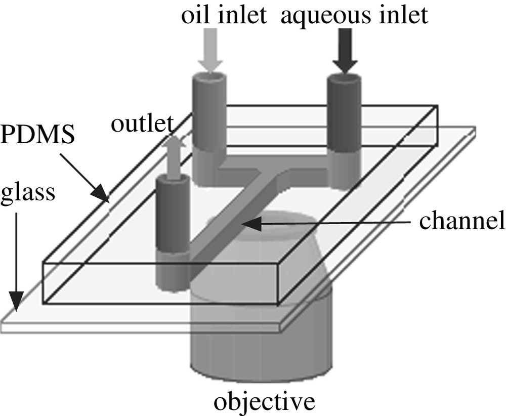
Sketch of the glass–PDMS microfluidic chip used in this study. The two inlet arms are filled with two immiscible fluids whose flow rates are imposed by syringe pumps. Observation of the flow is done under a microscope and picture is recorded, thanks to a CCD camera.

Fig. 10 shows the flow pattern diagram obtained with a mixture of 50 wt% of water with SDS at 2 cmc and 50 wt% of glycerine as aqueous phase and hexadecane in a 100 μm × 100 μm microchannel. The viscosity of the aqueous phase is of 7 cP and the oil phase is of 3 cP. During the experiment, three typical flow patterns have been identified: droplets formed at the T junction (DTJ), parallel flows or jets (PF) and parallel flows which break into droplets inside the channel (DC). Droplets are obtained in the upper left corner of Fig. 10, i.e., at low water flow rates and substantial oil flow rates. Two kinds of regimes must be distinguished. In the DTJ regime represented by (○), droplets are not always produced with reproducibilty in size whereas in the DC regime (●), monodisperse droplets are produced. In the latter case, a parallel flow (i.e., a jet) takes place at the entrance of the channel and becomes unstable after a short distance, breaking up into droplets. In the lower right, corner jets are observed. To investigate the three dimensional structure of the flow, confocal fluorescence microscopy experiments are performed. In this case rhodamine (Sigma) is added to the aqueous phase and hexadecane is used as the oil phase. Fig. 11 displays cross-section images obtained for PF in a 100 μm × 100 μm microchannel. The channel walls represented here have been drawn and added to the picture. The bottom wall is in glass and the three others are in PDMS. At the entrance of the funnel, hexadecane starts wrapping around the water. This is due to the difference of wettability of the two fluids with the PDMS walls. The water flow cross-section continues evolving until the flow mainly evolves along the propagation axis. Depending on the flow rates, jets or DC are then observed. PF is a truncated cylinder jet located on the glass at the PDMS glass corner. The pressure in a cross-section is uniform inside each fluid and differs from one fluid to the other. The Laplace law imposes that the free fluid surface has a single curvature radius.

Fig. 10
Flow pattern diagram as a function of the aqueous phase flow rate (Q_water) and of the oil phase flow rate (Q_oil) in a 100 μm × 100 μm microchannel. The aqueous phase is a mixture of water with SDS (2 cmc) 50 wt% and of glycerine 50 wt%. The oil phase is hexadecane. The ○ refers to droplets formed at the T junction (DTJ), the ◊ to parallel flows (PF) and the ● to parallel flows that break into droplets inside the channel (DC).

Fig. 11
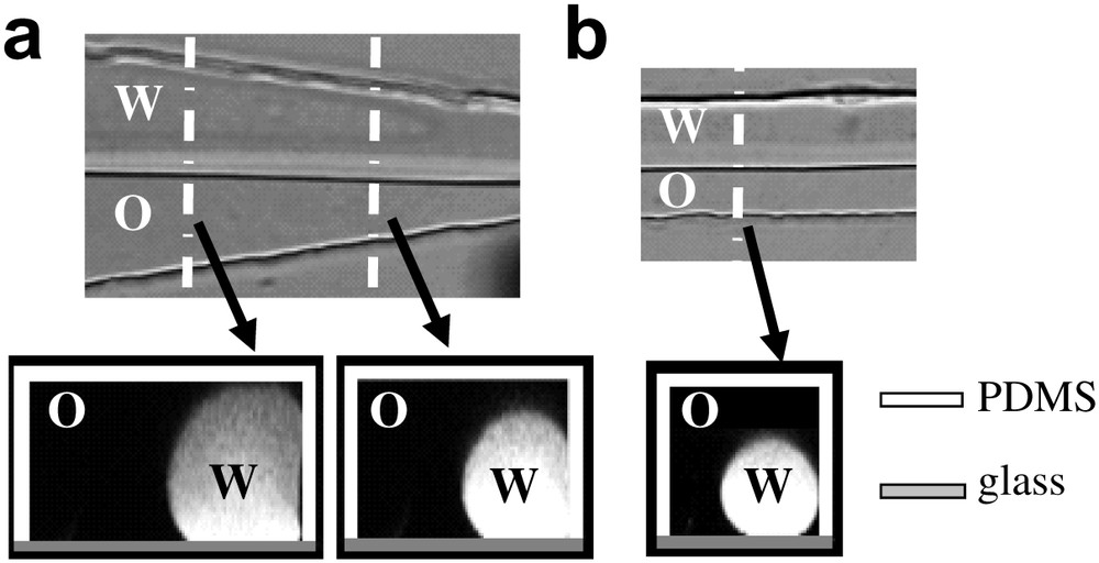
Cross-section picture of parallel flow between hexade-cane (O) and aqueous phase with rhodamine (W) in a 100 μm × 100 μm microchannel: (a) inside the funnel; (b) in the outlet channel.

5 Extension of our model to rectangular geometry

In this section, we try to extend the previous analysis to a microchannel with a rectangular cross-section. Two situations have to be analyzed. The inner jet may or may not be squeezed by the geometric confinement. We first focus on situations where the jet touches the upper and lower walls.

5.1 Squeezed jet in rectangular geometry

We consequently consider as the reference geometry a jet squeezed by the geometry. We assume that the contact angle θ between the internal and external phases on the glass is constant. In the unperturbated state, the free fluid–fluid interface has a shape involving a single radius curvature (see Fig. 12).

Fig. 12
Schematic representation of a non squeezed and a squeezed jet.

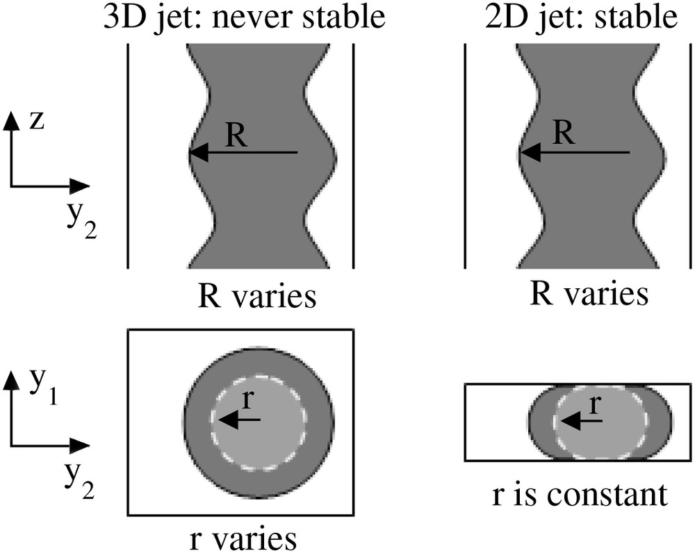
We wish to analyze again the stability of such a jet to axial perturbations without having to move to 3D numerical simulations. We therefore proceed with an uncontrolled approximation and consider only axially symmetric perturbations of the radius of the jet independent of the polar angle. In the small perturbations case and for a squeezed jet, the perturbated jet remains squeezed by the geometric confinement. This point is very important, since it sets the shape of the perturbations. Indeed, it ensures that the curvature radius remains constant in the geometry cross-section. The first term in the Laplace equation (Γ∂_zδr_i) is thus nil. As a consequence the dispersion equation in the approximation of the lubrication reads:

\tilde{ω} = \frac{- i \tilde{k} \cdot x^{3} Ka E (x) - F (x) ({\tilde{k}}^{4})}{D (x)} .

(16)

All ω_rs are negative and the 2D jet is thus stable. Confining the jet and squeezing it thus ensures its stability. Perturbations leading to the interfacial area reduction are unable to develop. The same results have been previously derived by Miguel et al. [32]. Note also that this scenario of stable “2D” jet where the area reduction is killed by the confinement had been experimentally shown by Dollet et al. [33] in a flow focusing design. This results explain why coflow situations are often encountered in microfluidic devices [13,34].

5.2 Non-squeezed jet in rectangular geometry

We now deal with situations where the jet is not squeezed by the wall. The flow studied is a wetting jet on the glass plate as observed in confocal experiments. In our calculation we will only consider axisymmetric perturbation of the radius of the jet. We assume that the contact angle θ between the internal and external phases on the glass is constant. With this assumption the center of the jet depends on the radius r and θ as depicted in Fig. 13.

Fig. 13
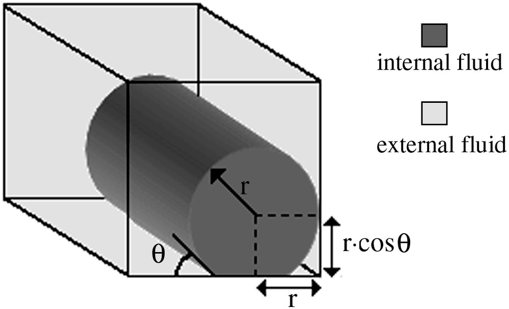
Flow geometry used in the simulation. The internal phase is a cylinder of radius r which wets a wall with a constant angle θ. θ is assumed to be constant with the flow rates. The center of the cylinder depends only on the radius r and on the contact angle θ.

To calculate the front velocity of the propagation we need to calculate the variation of the internal flow rate δQ_i and the external one δQ_e as a function of a small variation of the radius (δr) and of the pressure in both fluids (δP_e and δP_i):

δ Q_{e} = \frac{\partial Q_{e}}{\partial \nabla P_{e}} \partial δ P_{e} + \frac{\partial Q_{e}}{\partial \nabla P_{i}} \partial δ P_{i} + \frac{\partial Q_{e}}{\partial r} \partial δ r

(17)

δ Q_{i} = \frac{\partial Q_{i}}{\partial \nabla P_{e}} \partial δ P_{e} + \frac{\partial Q_{i}}{\partial \nabla P_{i}} \partial δ P_{i} + \frac{\partial Q_{i}}{\partial r} \partial δ r

(18)

where ∇P_e and ∇P_i are the pressure gradients in the internal and external phases, respectively.

The flow rates are numerically calculated using the Stokes equation in the geometry of Fig. 13. The boundary condition used is no-slip at the wall and the continuity of the velocity and of the shear stress at the fluid–fluid interface [35,36]. Calculations are made using the scientific software Scilab developed by INRIA. The numerical procedure used to calculate the flow profile is described in precision elsewhere [37]. We used a Cartesian regular mesh whose size is 1 μm × 1 μm. To calculate the different terms of Eqs. (17) and (18) we calculate the flow rates for both fluids for the different conditions described in Fig. 14. We calculate then the flow rates at the transition between the absolute and convective instabilities for different pressure gradients.

Fig. 14
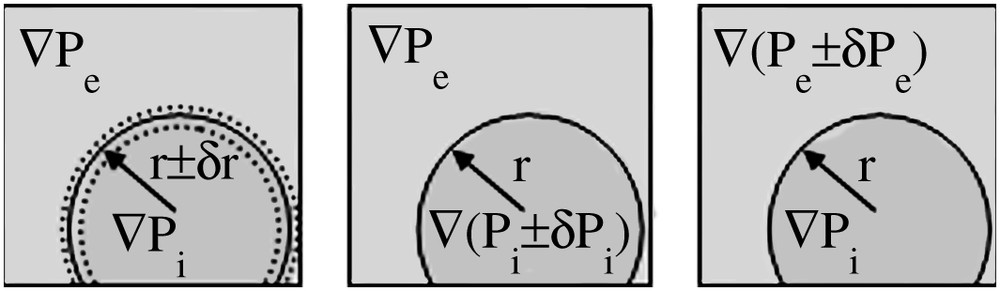
Variation of the parameters made in the numerical simulation. Each paramaters (r, P_e and P_i) are slightly varied by keeping the others constant. Both flow rates (Q_i and Q_e) are numerically calculated in each situation. This allows calculating the partial derivative of the flow rates with r, P_e and P_i in Eqs. (17) and (18).

6 Comparison with experimental data

The absolute/convective transition is calculated taking into account the geometry of the channel, the viscosity of both phases and the contact angle θ measured either by confocal microscopy pictures or by the transmission picture (to precision on this measure see Ref. [37]). Fig. 15 shows results with silicone oil sytems. Lines are theoretical transitions between absolute and convective and symbols (● and ○) are experimental transitions obtained for two viscosities (100 mPa s and 50 mPa s) and two surface tensions (Γ = 15 mN/m and Γ = 30 mN/m).

Fig. 15
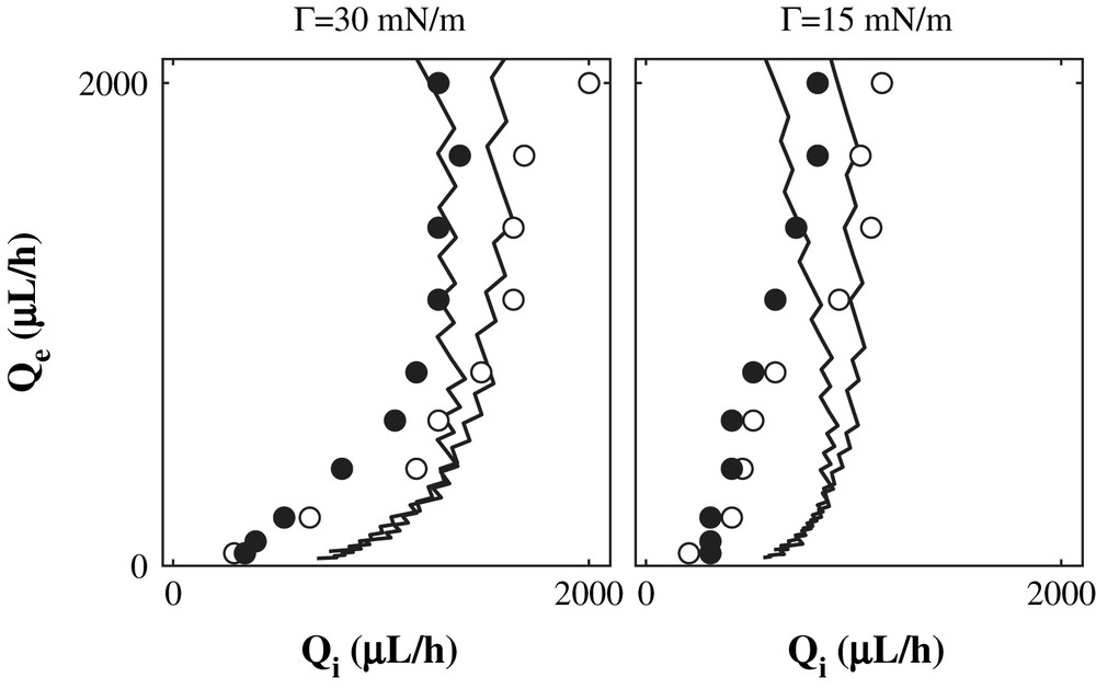
Transition between droplets and parallel flows for silicone oil system. Lines correspond to the transition from absolute to convective instability obtained by numerical simulations. Symbols are experimental transitions for silicone oil at 100 mPa s (●) and at 50 mPa s (○). The aqueous phase is a mixture of glycerine and water at 11 mPa s with (Γ = 15 mN/m) or without (Γ = 30 mN/m) SDS.

Results are in good agreement without any adjustable parameter and the theoretical transitions move in the same way as the experimental ones. The same conclusions are reached when the external phase is hexadecane with (◊) and without () Span 80 (see Fig. 16). When the internal phase viscosity is changed to 7 mPa s, good agreement is obtained with hexadecane (), silicone oil at 20 mPa s (▾) and 100 mPa s (●).

Fig. 16
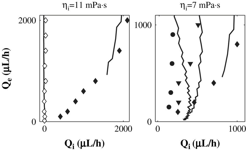
Transition between droplets and parallel flows for two different internal phases with SDS at 11 mPa s and 7 mPa s. Lines correspond to the transition from absolute to convective instability obtained by numerical simulation. Symbols are experimental transitions at Γ = 15 mN/m for hexadecane (), silicone oil at 100 mPa s (●) and at 20 mPa s (▾). To decrease the surface tension towards Γ = 1 mN/m we added span 80 in hexadecane (◊).

7 Conclusion

In this work, using the lubrication approximation and focusing on low Reynolds numbers, we have studied the stability of a pressure-driven jet confined in a capillary. Analyzing the transition from a continuous jet to a dripping system in terms of a convective/absolute transition, we find the jet remains continuous at high capillary numbers and breaks down into droplets at lower flow rates, i.e., pressure gradients. Analytical formulas are provided in cylindrical capillaries for a given system where viscosities and surface tension are known. The influence of the various system and operation parameters has been highlighted. At the expense of further approximations, we have explored other microchannel geometries, that are more relevant in the microfluidics context given fabrication processes. Microchannels of rectangular cross-section promote droplets at strong confinement when contrasted with their cylindrical counter-parts, most likely because corners allow easier fluid transfer. The outlook deals with the modelization of the volume of the droplets. Numerical simulations using level set methods are under way in order to address this problem.

Bibliographie

[1] P.G. de Gennes C. R. Acad. Sci., 326 (1998) no. 5, p. 331

[2] S.L. Anna; N. Bontoux; H.A. Stone Appl. Phys. Lett., 87 (2003), p. 364

[3] A.S. Utada; E. Lorenceau; D.R. Link; D.W. Weitz Science, 308 (2005), p. 537

[4] T. Nisisako; S. Okushima; T. Torii Soft Matter, 1 (2005), p. 23

[5] T. Nisisako; T. Torii; T. Higuchi Chem. Eng. J., 101 (2004), p. 23

[6] H. Song; R.F. Ismagilov J. Am. Chem. Soc., 125 (2003) no. 47, p. 14613

[7] P. Laval; N. Lisai; J.-B. Salmon; M. Joanicot Lab Chip, 7 (2007), p. 829

[8] P. Laval; J.-B. Salmon; M. Joanicot J. Cryst. Growth, 303 (2007), p. 622

[9] B. Zheng; J.D. Tice; R.F. Ismagilov Anal. Chem., 76 (2004), p. 4977

[10] T.M. Squires; S.R. Quake Rev. Mod. Phys., 77 (2005), p. 977

[11] P.G. de Gennes Rev. Mod. Phys., 57 (1985), p. 827

[12] R. Dreyfus; P. Tabeling; H. Willaihme Phys. Rev. Lett., 90 (2003), p. 144505

[13] P. Guillot; A. Colin Phys. Rev. E, 72 (2005), p. 066301

[14] P. Garstecki; M.J. Fuerstman; H.A. Stone Lab. Chip., 6 (2006), p. 437

[15] M. de Menech; P. Garstecki; F. Jousse; H.A. Stone J. Fluid Mech., 595 (2008), p. 141

[16] I. Vihinen; A.M. Honohan; S.P. Lin Phys. Fluids, 9 (1997), p. 3117

[17] A.P.R. Edwards; B.P. Osborne; J.M. Stoltzfus; T.A. Steinberg Phys. Fluids, 14 (2002), p. 3432

[18] M. Gordillo; J.N. Pérez-Saborid; A.M. Gañán-Calvo J. Fluid Mech., 23 (2001), p. 448

[19] A. Sevilla; M. Gordillo; C. Martinez-Bazán Phys. Fluids, 14 (2002), p. 3028

[20] M. Gordillo; Z. Cheng; A.M. Gañán-Calvo; M. Marquez; D.A. Weitz Phys. Fluids, 16 (2004), p. 2828

[21] A. Sevilla; M. Gordillo; C. Martinez-Bazán Phys. Fluids, 17 (2005), p. 018105

[22] A.M. Gañán-Calvo; P. Riesco-Chueca J. Fluid Mech., 75 (2006), p. 553

[23] A.M. Gañán-Calvo; M.A. Herreda; P. Garstecki Phys. Rev. Lett., 96 (2006), p. 124504

[24] A.S. Utada; A. Fernandez-Nieves; J.M. Gordillo; D.A. Weitz Phys. Rev. Lett., 100 (2008), p. 014502

[25] P. Guillot; A. Colin; A.S. Utada; A. Ajdari Phys. Rev. Lett., 99 (2007), p. 104502

[26] T.R. Powers; D. Zhang; R.E. Goldstein; H.A. Stone Phys. Fluids, 10 (1998), p. 1052

[27] W.V. Saarloos Phys. Rev. A, 39 (1989), p. 6367

[28] W.V. Saarloos Phys. Rev. A, 37 (1989), p. 211

[29] T.R. Powers; R.E. Goldstein Phys. Rev. Lett., 78 (1997), p. 2555

[30] A.M. Gañán-Calvo Phys. Rev. E, 75 (2007), p. 027301

[31] D.C. Duffy; J.C. McDonald; O.J.A. Schueller; G.M. Whitesides Anal. Chem., 70 (1998), p. 4974

[32] M. San Miguel; M. Grant; J.D. Gunton Phys. Rev. A, 31 (1985), p. 1001

[33] B. Dollet; W. van Hoeve; J.-P. Raven; P. Marmottant; M. Versluis Phys. Rev. Lett., 100 (2008), p. 034504

[34] T. Thorsen; R.W. Roberts; F.H. Arnold; S.R. Quake Phys. Rev. Lett., 86 (2001), p. 4163

[35] E. Guyon; J.-P. Hulin; L. Petit; C.D. Mitescu Physical Hydrodynamics, Oxford University Press, 2001

[36] R.B. Bird; W.E. Stewart; E.N. Lightfoot Transport Phenomena, Wiley, 2002

[37] P. Guillot; P. Panizza; J.-B. Salmon; M. Joanicot; A. Colin; C.-H. Bruneau; T. Colin Langmuir, 22 (2006), p. 6438

Commentaires - Politique

Ces articles pourraient vous intéresser

Multiphase flows in microfluidics

Charles N. Baroud; Hervé Willaime

C. R. Phys (2004)

Two-phase flow patterns and size distribution of droplets in a microfluidic T-junction: Experimental observations in the squeezing regime

Yassine Mahdi; Kamel Daoud; Lounès Tadrist

C. R. Méca (2017)

A Soft Landing Approach for the Centrifugal Microgel Synthesis Process

Matei Badalan; Lucie Adisson; Arthur Boldron; ...

C. R. Méca (2023)