Effects of salinity and temperature coupling on solid/liquid equilibria: Thermodynamic bases

Mireille Privat

doi:10.1016/j.crci.2009.01.004

Résumés

Anglais
Français

The basic rules of thermodynamics are applied to phase equilibria to describe the variations of solubility induced by changes in salinity and temperature in the case of a solid compound that separates pure (no solid solution). Even though the one or the other of these effects has been the subject of numerous investigations, those about the conjunction of both parameters are scarce and (almost) empirical despite the increase in the frequency of occurrence of practical cases, especially in biology and in the environment. This thermodynamic survey includes a rigorous treatment accompanied with possible approximations allowing one to get a prediction tool from a limited number of experimental parameters. The systems of concentration variables and reference states in current use are taken into account.

Cette présentation utilise les règles de base de la thermodynamique des équilibres de phase pour décrire l'évolution de la solubilité d'un solide en fonction à la fois de la température et de la salinité, dans le cas où le solide se sépare de la solution sous forme pure. Si de nombreuse études ont été faites sur l'effet de l'un ou l'autre de ces facteurs, leur effet conjugué a été rarement traité et le plus souvent de façon empirique malgré l'occurrence de plus en plus fréquente de cas pratiques dans des domaines aussi divers que la biologie ou l'environnement. Cette étude thermodynamique comporte un traitement rigoureux et indique les approximations possibles pour obtenir des formules utilisables comme outil prédictif à partir d'un nombre réduit de paramètres expérimentaux. Les différents systèmes de variables de composition et d'états de référence sont pris en compte.

1 Introduction

The solubility behaviours of a large variety of compounds are of key importance in many natural processes or in fields of activities by humans. For some time, attention has been focused on the solubility of gases such as carbon dioxide or dioxygen in freshwaters as well as in salted ones, e.g. human blood [1,2]. The dissolution and re-precipitation of solid compounds, e.g. calcium carbonate (calcite, aragonite, …), between rocks and water [3,4] or between bones and biological fluids [5–7] are of great concern in geology as well as in pathological sciences. Attention has been recently focused on the physical outcome of cargos accidentally spilled because of shipwreck or other sea event [8–12]. It is, indeed, worth wondering about their fate: indeed, in the event of dissolution of a certain part of a given cargo, which will be this part and in which amount? Is this amount dependent upon temperature and/or water salinity? What is its time evolution?

The literature contains many descriptions of the solubility phenomenon plus others about the effects of either salinity [13–20] (this in a rather phenomenological way) or temperature [1,2,21]. However, to our knowledge, until now no rigorous and synthetic study of the combination of both effects has been reported in the literature. Moreover, most of the people in charge of field measurements have no background in thermodynamics, though they need a precise knowledge of the basic rules that would allow them to correctly use literature data and make the possible, and sometimes necessary, approximations.

Concerning the present and preliminary study, focus will be on only the dissolution/precipitation of solids in more or less salted water and in the simple case where the solid separates pure (no solid solution). Indeed, this simplification of the question under study is not only helpful, but also relevant because it corresponds to many practical cases. The rules governing the behaviour of the dissolution/separation of partially soluble liquid compounds are fundamentally the same, but the formalism is more complicated because the composition of the phase that separates at the solubility limit varies with salinity and/or temperature. This case study will be presented later in another report.

About the restricted case mentioned previously and on condition of knowing the solubility at a single salinity–temperature couple, our aim is to propose a way to calculate the solubility of a solid at any salinity and temperature from some other physical properties of the system. Several possible approximations will be also proposed.

2 Fundamental law of phase equilibria

Let us consider a liquid solvent, A₁, and a compound, A₂. At a given temperature, the equilibrium between the pure solid state of A₂ and its state in solution in A₁ can be written as expressed in Eq. (1) [21,2] on condition to consider A₁ as a simple liquid solvent or a liquid mixture, e.g. water and salt:

A_{2} (c) = A_{2} (ℓ, sal)

(1)

where c is the solid (crystal) state, ℓ is the liquid state and “sal” is the salinity. One should note that, in the following, “sal” will be usually expressed either as the mole fraction, x₃ (for the basic thermodynamic treatment) or in mol L⁻¹; moreover, the dissolved salt will be assumed to never reach its own solubility limit, and the pressure will be set at a value such that the only phase equilibrium to be considered will be that described by Eq. (1). So, the system under study will in fact consist of three components (solvent 1, dissolved salt 3 and compound 2 at its solubility limit). There will be only 2 phases (ℓ and c), and on condition to set the pressure at, for example, 1 bar, the temperature will be the only intensive state variable. Then, the system variance will be:

V = n + 1 - φ = 3 + 1 - 2 = 2

(2)

which means two independent state variables, chosen here as salinity and temperature. Fixing one of them leads to a representation of the equilibrium expressed in (1) as a single line in a partial phase diagram where the composition of the liquid phase is shown versus the kept other variable. Let us denote sal₁ and T₁ the values of salinity and temperature at the start, and sal₂ and T₂, the values at the end. To pass from (sal₁ and T₁) to (sal₂ and T₂) one can follow, at first, the coexistence curve at constant T₁ up to sal₂, then, pass along the coexistence curve at constant sal₂ to go from T₁ to T₂. The thermodynamic condition for the phase equilibrium (1) is then:

μ_{2} (c) = μ_{2} (ℓ, sal) .

(3)

In explicit form, it is written as:

g_{2}^{*, c} (T) = g_{2}^{*, ℓ} (T) + R T \ln [f_{2} (T, sal, x_{2}) x_{2} (T, sal)]

(4)

where g's are molar Gibbs free energies.

In Eq. (4), the superscript ^∗ reads for “pure”; the corresponding free energy then depends on both the temperature and pressure. But since at a pressure close to the atmospheric one, the dependence is weak, it allows one to omit the term, P, which should be enclosed in the brackets. More specifically, this is also consistent with the hypothesis of a constant pressure. About f₂, it is the activity coefficient defined with respect to a reference state chosen as the pure component, 2 (x₂ = 1); f₂ tends to 1 when x₂ tends to 1. It is worth noting that, on condition the pressure be close to 1 bar and the reference state be the pure component, the symbol ^∗ can be replaced by the symbol of the standard state,⁰.

Another reference state like, for instance, the ideal solution corresponding to the infinitely dilute solution may be chosen in solution. Then, Eq. (4) becomes:

g_{2}^{*, c} (T) = g_{2}^{θ x, ℓ} (T) + R T \ln [γ_{2}^{x} (T, sal, x_{2}) x_{2} (T, sal)]

(4′)

where γ₂^x is the activity coefficient with respect to the ideal state, with the constraint γ₂^x tending to 1 when x₂ tends to 0.

g_{2}^{θ x, ℓ}

is the corresponding standard form.

But, if the composition variable is molarity, Eq. (1) becomes:

g_{2}^{*, c} (T) = g_{2}^{θ c, ℓ} (T) + R T \ln [γ_{2}^{c} (T, sal, c_{2}) c_{2} (T, sal)]

(5)

where γ₂^c is then the activity coefficient with respect to the ideal state, with the constraint γ₂^c tending to 1 as c₂ tends to 0. This form of writing the chemical potential is useful when the Setchenov rule is used to express the salinity dependence of the activity coefficient of compound 2. On the other hand, when the investigations deal with the influence of temperature, Eqs. (4) and (4′) have to be preferred because the definition of x₂ implies no additional effect by temperature conversely to c₂. As usual, the choice of the expression for μ₂ is only a question of convenience.

When Eq. (4) is used, the solubility appears as a mole fraction, whereas with Eq. (5) it appears as a molarity. Once obtained, any of these values can be easily converted into the other one.

One should also note that comparing Eqs. (4) and (4′) leads to:

R T \ln (γ_{2}^{x} / f_{2}) = g_{2}^{*, ℓ} - g_{2}^{θ x, ℓ}

(6)

3 Evolution of solubility with salinity, at constant temperature. Role of the Setchenov equation

3.1 Form of the phase diagram

Addition of salt to a three-component mixture (water, solute and salt respectively denoted 1, 2 and 3) at a constant temperature, T, induces changes in the concentrations of all of the three components of the system, x₁, x₂, and x₃, respectively. So, from a general point of view, it is a rule to represent the phase equilibrium line in a triangular diagram such as that in Fig. 1a. The pure solid phase, 2, is in equilibrium with every saturated solutions; so as shown in Fig. 1a, all of the solid–liquid tie lines converge at the point (x₂ = 1, x₁ = x₃ = 0). The dotted area corresponds to the case where, in practice, the system undergoes a maximum salinity value, denoted sal_max in this figure: for example, the maximum salinity for the sea-water or biological fluids like blood corresponds to a mole fraction around 0.01. The values in the dotted area may correspond to various situations such as those observed in an estuary. Fig. 1b displays the ordinary representation (solubility–salinity) denoted (sol, sal), which is right according to thermodynamics, but less friendly user for fundamental analyses. However, this kind of drawing is the most common representation of experimental data. In most of the cases, molarities are used instead of mole fractions, but the latter are mentioned in Fig. 1b as possible options in order to facilitate comparisons of Fig. 1a and b. The dotted area on Fig. 1b indicates the area where the salinity can be the highest depending on the specificity of the medium under study (e.g. sea-water). Fig. 1a and b constitutes not only a useful visual summary of the effects by the thermodynamic variables on solubility, but also a reminder of the definitions used in the equations below.

Fig. 1
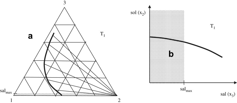
(a) Solubility line at constant temperature for a component 2 separating as pure solid from a mixture with water (component 1) and salt (component 3), in a triangular representation. Tie lines with the pure component 2 are shown as well as the area where salted water may be found in the environment; sal_max is the mean salinity of the sea-water as well as of biological tissues such as the blood. The variation of solubility when salinity x₃ is raised corresponds to a “salting-out” (it decreases). (b) The same solubility line in an orthogonal representation.

3.2 Equation of the equilibrium line using the mole fraction scale

Equation (4) gives the most straightforward way to get the solubility under the form of a mole fraction:

x_{2} (T, sal) = [1 / f_{2} (T, sal, x_{2})] \exp {[[g_{2}^{*, c} (T) - g_{2}^{*, ℓ} (T)] / R T]}

(7)

x_{2} (T, sal) = [1 / f_{2} (T, sal, x_{2})] \exp {[- [Δ_{fus} g_{2}^{*} (T)] / R T]}

(8)

where Δ_fusg₂^* is the free energy of fusion of the pure component 2.

In pure solvent, Eq. (8) becomes:

x_{2}^{0} (T, sal = 0) = [1 / f_{2}^{0} (T, sal = 0, x_{2}^{0})] \exp {[- [Δ_{fus} g_{2}^{*} (T)] / R T]}

(9)

where x₂⁰ is the solubility in pure solvent.

Then the ratio between Eqs. (9) and (8) leads to:

[x_{2}^{0} (T, sal = 0)] / [x_{2} (T, sal)] = [f_{2} (T, sal, x_{2}) / f_{2}^{0} (T, sal = 0, x_{2}^{0})]

(10)

The empirical Setchenov equation is written as:

\log_{10} [x_{2}^{0} (T, sal = 0)] / [x_{2} (T, sal)] = K_{x}^{S} x_{salt}

(11)

where K_x^S is the so-called Setchenov constant if mole fractions are used, and x_salt is the mole fraction of salt in the solution (sal). All Setchenov constants depend on the natures of salt 3 and solute 2. Moreover, Eq. (10) indicates that

K_{x}^{S} x_{salt} = \log_{10} [f_{2} (T, sal, x_{2}) / f_{2}^{0} (T, sal = 0, x_{2}^{0})]

(11′)

which gives a thermodynamic sense to the Setchenov constant.

Equation (10) clearly shows that the solubility ratio directly depends on the activity coefficients, which in turn depend on the concentration of component 2, salinity and temperature. Relation (10) can be expressed in a different way by using the same method as previously from equation (4′) at first for salted solutions and then for solutions in pure solvent. On condition of denoting as Δ_fusg₂^θx the standard free energy in the present state of reference, one gets:

x_{2} (T, sal) = [1 / γ_{2}^{x} (T, sal, x_{2})] \exp {[- [Δ_{f u s} g_{2}^{θ x} (T)] / R T]}

(12)

x_{2}^{0} (T, sal = 0) = [1 / γ_{2}^{x} (T, sal = 0, x_{2}^{0})] \exp {[- [Δ_{fus} g_{2}^{θ x} (T)] / R T]}

(12′)

[x_{2}^{0} (T, sal = 0)] / [x_{2} (T, sal)] = [γ_{2}^{c} (T, sal, x_{2}) / γ_{2}^{c 0} (T, sal = 0, x_{2}^{0})]

(13)

\log_{10} [x_{2}^{0} (T, sal = 0)] / [x_{2} (T, sal)] = \log_{10} [γ_{2}^{x} (T, sal, x_{2}) / γ_{2}^{x 0} (T, sal = 0, x_{2}^{0})] = K_{x}^{s} x_{salt}

(14)

The interest of these relations is that, in dilute solutions, the activity coefficients tend to 1; this is often the case for saturated solutions when the salt is missing. It ensues that γ₂^x⁰ ∼ 1; this is why the solubility ratio is often described as the activity coefficient of solute 2 in a saline solution and why the Setchenov relation may be considered as an empirical expression of this activity coefficient.

However, few data about this dependence have been obtained within this scale of compositions (x₂), and the use of molarity may appear as offering more user-friendly relationships and corresponds, in fact, to richer series of experimental data [5,8–11]. When some of them are expressed in g L⁻¹, they are easily converted into molarities.

3.3 Equation of the equilibrium line using the molarity scale

Use of Eq. (5) as a basis and application of a treatment similar to the one in Eqs. (12)–(14) lead to the following expression of Setchenov relationship in mol L⁻¹:

\log_{10} [c_{2}^{0} (T, sal = 0)] / [c_{2} (T, sal)] = \log_{10} [γ_{2}^{c} (T, sal, c_{2}) / γ_{2}^{c 0} (T, sal = 0, c_{2}^{0})] = K_{c}^{S} c_{salt}

(15)

where K_c^S is the Setchenov constant in this scale of composition.

In dilute solutions, as these activity coefficients tend to 1, a common approximation is γ₂^c⁰ ∼ 1. Then, the solubility ratio gives the activity coefficient in saline solution, and the Setchenov equation provides one with its empirical expression (see Section 3.2).

When the mixture under study consists of electrolytes, it is worth recalling that relation (15) becomes [1]:

\log_{10} [c_{2}^{0} (T, sal = 0)] / [c_{2} (T, sal)] = K_{c}^{S'} I

(16)

where

K_{c}^{S'}

is the sum of individual salt-effect parameters for each salt and I is the ionic force, here expressed from molarities.

3.4 Possible approximations and practical use of these relations

Equations (14) and (15) can be replaced with Eqs. (14′) and (15′). At this stage, Eqs. (11) and (14′) are alike:

\log_{10} [x_{2}^{0} (T, sal = 0)] / [x_{2} (T, sal)] = K_{x}^{S} x_{salt}

(14′)

\log_{10} [c_{2}^{0} (T, sal = 0)] / [c_{2} (T, sal)] = K_{c}^{S} c_{salt}

(15′)

They show that determining solubility in pure solvent and at several salinity values allows one to determine K_z^S and then to get, by interpolation, solubility values at other salinities.

Eqs. (14) and (15), by the use of Eq. (10), write as well:

\log_{10} [γ_{2}^{x} (T, sal, x_{2}) / γ_{2}^{x 0} (T, sal = 0, x_{2}^{0})] = K_{x}^{S} x_{salt}

(14″)

\log_{10} [γ_{2}^{c} (T, sal, c_{2}) / γ_{2}^{c 0} (T, sal = 0, c_{2}^{0})] = K_{c}^{S} c_{salt}

(15″)

On condition the following approximation, γ₂^x⁰ ∼ 1 or γ₂^c⁰ ∼ 1, be valid and Eq. (5) be taken into account, Eqs. (14) and (15) can be rewritten as:

K_{x}^{S} x_{salt} = \log_{10} [γ_{2}^{x} (T, sal, x_{2})] = (1 / 2.303) {\ln [1 / x_{2} (T, sal)] - [Δ_{fus} g_{2}^{θ x} (T)] / R T}

(14‴)

K_{c}^{S} c_{salt} = \log_{10} [γ_{2}^{c} (T, sal, c_{2})] = (1 / 2.303) {\ln [1 / c_{2} (T, sal)] - [Δ_{fus} g_{2}^{θ c} (T)] / R T}

(15‴)

These equations show that, when the solubility of the solid in pure solvent is small enough, K_z^S depends only on the temperature. This result, which was found experimentally in [9], of course depends on the nature of the salt and solute under study [9,15,22,23].

To avoid experiments one may be tempted to use the thermodynamic data reported in the available Tables, which sometimes give also the standard free energy of fusion. Another way is to transform these data from:

- Δ_{fus} g_{2}^{θ x} (T) = g_{2}^{* c} (T) - g_{2}^{θ ℓ} (T) = [g_{2}^{* c} (T) - g_{2}^{o v} (T)] + [g_{2}^{o v} (T) - g_{2}^{θ ℓ} (T)] = - Δ_{sub} g_{2}^{*} (T) - R T \ln H_{2} (T)

(17)

where Δ_subg₂^*(T) is the sublimation free energy of pure component 2, and H₂(T) is the Henry constant of this component, H₂(T) = p₂/x₂^ℓ, in a very dilute solution of the solvent under study (p₂ is the partial vapour pressure, which can be determined from the concentration of vapour). The availability of new analytical techniques allows the determination of this constant with the precision required by certain applications [23–25]. The tables of thermodynamic data contain many Δ_fusg₂^∗, Δ_fusg₂^θx and Δ_fusg₂^θ^c as well as Henry's constants. Finally, the solubilities can be expressed as:

x_{2} (T, sal) = \exp {- 2.303 K_{x}^{S} x_{salt} - Δ_{fus} g_{2}^{θ x} (T) / R T}

(14″″)

c_{2} (T, sal) = \exp {- 2.303 K_{c}^{S} c_{salt} - Δ_{fus} g_{2}^{θ c} (T) / R T}

(15″″)

4 Evolution of solubility with temperature, at constant salinity

4.1 Basic treatment

This part of fundamental thermodynamics about the solubility of solid compounds is quite classical; it is particularly simple when none of the concentration variables, e.g. mole fraction and molality, structurally depends on the temperature.

On condition to use the same approximations as in Section 3, namely: (i) P set at a constant value and (ii) the solid phase containing only component 2, and on condition to also set salinity at a constant value while varying the temperature, the variance is again 1. In the phase diagram, the equilibrium is described by a line, and its equation can be found from Eq. (4).

From relation (8) written as follows:

\ln [f_{2} (T, sal, x_{2}) x_{2} (T, sal)] = g_{2}^{*, c} (T) - g_{2}^{*, ℓ} (T) = - Δ_{fus} g_{2}^{*} (T) / R T

(18)

one may take the derivative with respect to the temperature on both sides of the equation. Application of the Gibbs–Helmholtz equation to the term representative of fusion free energy leads to:

(\partial / \partial T) {\ln [f_{2} (T, sal, x_{2}) x_{2} (T, sal)]} = Δ_{fus} h_{2}^{*} / R T^{2}

(19)

Integrating between temperatures T₁ and T₂ leads to:

\ln {f_{2} [T_{2}, sal, x_{2} (T_{2})] x_{2} (T_{2}, sal)} - \ln {f_{2} [T_{1}, sal, x_{2} (T_{1})] x_{2} (T_{1}, sal)} = \int_{T 1}^{T 2} (Δ_{fus} h_{2}^{*} / R T^{2}) ⅆ T

(20)

The calculation of solubility data at any temperature, T₂, from data at T₁ requires to evaluate the activity coefficients from:

f_{2} (T_{2}, x_{1}, x_{2}, x_{3}) = f_{2} (T_{1}, x_{1}, x_{2}, x_{3}) \exp [\int_{T 1}^{T 2} {\bar{H}}_{2}^{e x} (T, x_{1}, x_{2} x_{3})] ⅆ T

(20′)

where

{\bar{H}}_{2}^{e x} (T, x_{1}, x_{2}, x_{3})

is the partial molar excess enthalpy of component 2 (note that x₃ ≡ sal).

Now, from Eq. (4′) one can write that:

\ln [γ_{2}^{x} (T, sal, x_{2}) x_{2} (T, sal)] = g_{2}^{*, c} (T) - g_{2}^{θ x, ℓ} (T) = - Δ_{fus} g_{2}^{θ x} (T) / R T

(21)

and so

(\partial / \partial T) {\ln [γ_{2}^{x} (T, sal, x_{2}) x_{2} (T, sal)]} = Δ_{fus} h_{2}^{θ x} (T) / R T^{2}

and by integration

\ln {γ_{2}^{x} [T_{2}, sal, x_{2} (T_{2})] x_{2} (T_{2}, sal)} - \ln {γ_{2}^{x} [T_{1}, sal, x_{2} (T_{1})] x_{2} (T_{1}, sal)} = \int_{T 1}^{T 2} (Δ_{fus} h_{2}^{θ x} / R T^{2}) ⅆ T

(22)

Similarly, from Eq. (5), one gets:

(\partial / \partial T) {\ln [γ_{2}^{c} (T, sal, c_{2}) c_{2} (T, sal)]} = Δ_{fus} h_{2}^{θ c} / R T^{2}

(23)

This equation contains some subtle temperature effects issued from the simple effect of temperature on molarity, i.e. with no change in the solution content.

However, in short ranges of temperature, one can write

\ln {γ_{2}^{c} [T_{2}, sal, c_{2} (T_{2})] c_{2} (T_{2}, sal)} - \ln {γ_{2}^{c} [T_{1}, sal, c_{2} (T_{1})] c_{2} (T_{1}, sal)} = \int_{T 1}^{T 2} (Δ_{fus} h_{2}^{θ c} / R T^{2}) ⅆ T

(24)

4.2 Empirical treatments and common approximations

When the interval of temperatures between T₁ and T_2, (T₂ − T₁), is small enough, a common approximation is to assume that Δ_fush₂^∗ is constant in Eq. (20), which allows one to express the integral on the right as:

\int_{T 1}^{T 2} (Δ_{fus} h_{2}^{*} / R T^{2}) ⅆ T \sim - (Δ_{fus} h_{2}^{*} / R) (1 / T_{2} - 1 / T_{1})

(25)

It is similar for Eq. (22):

\int_{T 1}^{T 2} (Δ_{fus} h_{2}^{θ x} / R T^{2}) ⅆ T \sim - (Δ_{fus} h_{2}^{θ x} / R) (1 / T_{2} - 1 / T_{1})

(26)

and Eq. (23)

\int_{T 1}^{T 2} (Δ_{fus} h_{2}^{θ c} / R T^{2}) ⅆ T \sim - (Δ_{fu s} h_{2}^{θ c} / R) (1 / T_{2} - 1 / T_{1})

(27)

According to experiments [16,9,1,2], when the Setchenov constant [Eqs. (14), (15), (14′), (15′), (14”), (15”)], is independent of concentrations, it is almost unaffected by temperature; this seems particularly true with metallic chlorides and between 25 and 40 °C [15,19]. Indeed the rare measurements of a temperature effect on the Setchenov coefficient have demonstrated a slight effect, but as they had been performed in the molarity scale, the observed effect may have been induced by the temperature-dependency of the molarity. It is true that, in a mixture, a massive presence of salts tends to dominate the interactions. So, it would be worth considering to what extent salt activity is temperature-dependent, since, at each step of temperature, it affects the activities of the other components.

It ensues that a possible approximation is:

K_{x}^{S} (T_{2}) \sim K_{x}^{S} (T_{1})

(28)

When the Setchenov approximation and Eq. (28) are both valid, salinity has only a slight effect upon the way the solubility of any compound is affected by temperature. Another way to reach the result is the following.

According to Eq. (11), when the salinity is weak and the solutions are dilute, $γ_{2}^{x} [T_{2}, sal, x_{2} (T_{2})] = γ_{2}^{x} [T_{1}, sal, x_{2} (T_{1})] = 1$ , and then the use of Eq. (22) leads to:

\ln {x_{2} (T_{2}, sal)} - \ln {x_{2} (T_{1}, sal)} = \ln {[x_{2}^{0} (T_{2}, sal = 0)]} - \ln {[x_{2}^{0} (T_{1}, sal = 0)]} = \int_{T 1}^{T 2} (Δ_{fus} h_{2}^{θ x} / R T^{2}) ⅆ T

(29)

Relation (29) means that the solubility varies with temperature and at constant salinity, “sal” = constant, it varies as in the absence of salt (“sal = 0”).

5 A proposal to evaluate solubility from data obtained at other salinity and temperature values

Fig. 2 exhibits the way one can pass from a solubility value in the state 1 (sal₁, T₁) of the system to the solubility value in the state 2 (sal₂, T₂). The large-dashed line shows how one can, at first, follow the coexistence line at T₁ until reaching ${sal}_{1^{'}} \equiv {sal}_{2}$ (state 1′).

Fig. 2
Solubility surface obtained from figures such as Fig. 1a when the temperature is varied. The triangle of Fig. 1a is used at three temperatures; the solubility is assumed to be enhanced by the rise of temperature. A dashed line from point 1 to point 2 shows how a coexistence line, at constant temperature, can be followed from salinity sal₁ to salinity sal₂ (also called ${sal}_{1'}$ in the text), point 1′, then at constant salinity, by varying the temperature from the point 1′ (at T₁) to the point 2 (at T₂). Point 1 could have been chosen at salinity 0. A second path (dotted line) shows how, in a medium where salinity is spontaneously limited (e.g. sea-water), one can determine the solubility from a value at another salinity, even null.

The equation representative of the whole path can be written in either a rigorous way or in a simplified formulation as shown below.

5.1 Rigorous equation

The evolution of the solubility of component 2, at first along the path from state 1 to state 1′, is then described in the rigorous form by Eq. (10) or (11) in the symmetrical system of reference, or by Eq. (15) in the unsymmetrical system; one should note that Eqs. (11) and (15) include Setchenov's formula. Then, the changes in solubility between state 1′ and state 2 are described by Eq. (20) or (22) in the symmetrical system or the corresponding ones in the unsymmetrical system.

By using Eq. (10) to pass from state 1 (T₁, x₂¹, sal₁) to state 1′ (T₁, $x_{2}^{1'}$ , ${sal}_{1'}$ ), i.e. along an isotherm, then by using Eq. (20) along an “iso-salinity” path to go from state 1′ (T₁, $x_{2}^{1'}$ , ${sal}_{1'}$ ) to state 2 (T₂, x₂², ${sal}_{1'}$ ) one gets:

x_{2}^{2} = [f_{2} (T_{1}, x_{2}^{1}, {sal}_{1}) / f_{2} (T_{2}, x_{2}^{2}, {sal}_{1'})] x_{2}^{1} \exp [\int_{T 1}^{T 2} (Δ_{fus} h_{2}^{*} / R T^{2}) ⅆ T]

(30)

Both f₂ parameters can be estimated from Eq. (11′) written at T₁ and at T₂, respectively. So the ratio of activity coefficients in Eq. (30) writes:

\ln [f_{2} (T_{1}, {sal}_{1}, x_{2}^{1}) f_{2}^{0} (T_{2}, sal = 0, x_{2}^{0}) / f_{2} (T_{2}, {sal}_{1'}, x_{2}^{2}) f_{2}^{0} (T_{1}, sal = 0, x_{2}^{0})] = 2.303 [K_{x}^{S} (T_{1}) x_{sal} - K_{x}^{S} (T_{2}) x_{sal}^{'}]

(31)

where x_sal and

x_{sal}^{'}

are the molar fractions of salt in state 1 and in state 1′, respectively.

Combining Eqs. (30) and (31) leads to a rigorous equation expressed as:

x_{2}^{2} = x_{2}^{1} {\exp [K_{x}^{S} (T_{1}) (x_{sal}) - K_{x}^{S} (T_{2}) (x_{sal}^{'})]} [f_{2}^{0} (T_{1}, sal = 0, x_{2}^{0}) / f_{2}^{0} (T_{2}, sal = 0, x_{2}^{0})] \exp [\int_{T 1}^{T 2} (Δ_{fus} h_{2}^{*} / R T^{2}) ⅆ T]

(32)

By using the unsymmetrical reference system, this equation becomes:

x_{2}^{2} = x_{2}^{1} {\exp [K_{x}^{S} (T_{1}) (x_{sal}) - K_{x}^{S} (T_{2}) (x'_{sal})]} [γ_{2}^{0} (T_{1}, sal = 0, x_{2}^{0}) / γ_{2}^{0} (T_{2}, sal = 0, x_{2}^{0})] \exp [\int_{T 1}^{T 2} (Δ_{f u s} h_{2}^{θ x} / R T^{2}) ⅆ T]

(33)

On condition of admitting the Setchenov relationship, Eq. (33) rigorously describes the evolution of the solubility limit of a pure solid further to changes in temperature and salinity. In principle, this equation can be used in both senses: the known terms are either x₂¹, x₂² and Δ_fush₂^θx plus, for example, K_x^S, (left member of Eq. (33)), and then one gets information about γ₂⁰, or those on the right, and then the x₂² value can be calculated from x₂¹ one. This second case is the one met in accidental environmental events when practical solutions have to be found from partial data or had been previously included in codes written for decisional tools; then these codes must contain a sufficient amount of data to allow calculation. There is no doubt that getting the detailed knowledge of the physical characteristics (as contained in Eq. (33)) of any chemical liable to be implicated in accidental events remains impossible. So, it is worth using simplified relationships, such as those presented in the next paragraph, while being aware of their limitations deduced from comparison with Eq. (33).

One should, however, note that models able to calculate activity coefficients are available [1,2,26] and could be used in Eq. (33). Unfortunately, calculations are too time-consuming whenever measures have to be quickly taken because of an accidental event.

5.2 Dilute system, simplified Setchenov's formulation

In the absence of salt, when the solubility is low at both temperatures, γ₂⁰ at both temperatures can be approximated to 1. If, in addition, K_x^S is admitted to be temperature-independent, K_x^S (T₂) ∼ K_x^S (T₁) = K_x^S

If Δ_fush₂^θx does not depend on temperature or if (T₂ − T₁) is small, the integral can be also approximated, which leads to the following approximation of Eq. (33):

x_{2}^{2} = x_{2}^{1} {\exp [K_{x}^{S} (x_{sal} - x_{sal}^{'})]} \exp [- Δ_{fus} h_{2}^{θ x} (1 / T_{2} - 1 / T_{1})]

(34)

If the start of experiments, or calculation, is at null salinity, then x_sal = 0 and:

x_{2}^{2} = x_{2}^{1} {\exp [K_{x}^{S} (- {x'}_{sal})]} \exp [- Δ_{fus} h_{2}^{θ x} (1 / T_{2} - 1 / T_{f})]

(35)

Expressions (34) and (35) are far simpler than Eq. (33), and everyone knows exactly which approximations have been made to get them and, thus, when they have to be used in a more elaborated form.

In many cases, particularly when slightly soluble compounds are dissolving in the marine environment, the mole numbers contained in 1 L of mixture are clearly smaller for solutes than for water: n₂, n₃ ≪ n₁ ∼ (m₁/M₁) = 1000/18 = 55.5, and thus, n₂ ∼ c₂ and n₃ ∼ c₃, which leads to rewriting Eq. (34) as:

c_{2}^{2} = c_{2}^{1} {\exp [K_{x}^{S} (- {c'}_{sal} / 55.5)]} \exp [- Δ_{fus} h_{2}^{θ x} (1 / T_{2} - 1 / T_{f})]

(36)

Let us examine the Setchenov equation in molarity and mole fraction scales; respectively, it gives:

\log_{10} (c / c^{0}) = - K_{c}^{S} c_{salt}

(37)

\log_{10} (x / x^{0}) = - K_{x}^{S} x_{salt}

(38)

and by using the same approximation as above, one gets:

\log_{10} (x / x^{0}) = - K_{x}^{S} c_{salt} / 55.5 = \log_{10} [(c / 55.5) / (c^{0} / 55.5)] = - K_{c}^{S} c_{salt}

that is:

K_{x}^{S} / 55.5 = K_{c}^{S}

(39)

Then Eq. (36) becomes:

c_{2}^{2} = c_{2}^{1} {\exp [K_{c}^{s} (- {c'}_{sal})]} \exp [- Δ_{fus} h_{2}^{θ x} (1 / T_{2} - 1 / T_{f})]

(40)

It is worth noting that this expression uses molarities in each term except the enthalpy of fusion, which results from a rigorous analysis of temperature effects made impossible when direct molarities are used in the calculations.

Obviously, when salt effect is used in extraction processes, the salt concentrations are far too high to allow the use of these approximations. But, in the case of an accidental marine pollution by chemicals, Eq. (35), and above all Eq. (40), can provide one with a correct evaluation of the solubility under marine conditions at the very temperature of sea-water despite the dependency of this temperature on weather conditions and the period of the day (daylight against night). These formulae are worth using because the amount of data to be known is small: only are required the melting enthalpy at P = 1 bar, the melting temperature, T_f, and the Setchenov constant, K_x^S or K_c^S. The two first parameters are available in the Tables of thermodynamics, and if the Setchenov constants have not been measured, they can be calculated by incremental methods [10,16,20,22].

6 Conclusion

By using the fundamentals of thermodynamics about phase equilibria and the effect of salinity on the solubility limit of any solute proposed by Setchenov we established a relationship between the solubility at a first state of salinity and temperature (sal₁ and T₁) and the one in a second state (sal₂ and T₂). This relation may use mole fractions in the symmetrical system of reference (Eq. (32)) or in the unsymmetrical one (Eq. (33)). In dilute solutions including mixtures in sea-water, and on condition the variation of temperatures be small, these equations can be simplified (relations (35) and (36), respectively) in order to foresee realistic solubility values from only a set of essential parameters: the melting enthalpy and the melting temperature of the pure solute under study, the Setchenov coefficient. A less rigorous equation, namely Eq. (40), relies on the use of molarities. Among these essential parameters the two first one have to be found in Tables, whereas the third one has to be measured or estimated from increments found in literature. Some care has, however, to be taken with respect to the conversion of data from a system of concentrations to another one since molarities are more difficult to use in studies where temperature varies. Similarly, the reference systems for activity coefficients have to be taken into account. Then, the use of Henry's constants plays a fundamental role. When chemicals are characterised by unusual values of thermodynamic parameters, particularly high solubility values, coming back to the more elaborated relations in order to study specific treatments of the issue of concern is a must. The formalism used in the present study cannot be directly applied to any kind of solubility limit: in particular, it is inapplicable for two reasons when the pure form of the solute under study is liquid. Indeed, i) the phase that separates when the solution is saturated is a mixture, and ii) the parameter equivalent to the enthalpy of fusion becomes a transfer coefficient, and then it is less easily handled than the previous enthalpy.

Appendix Chemical potentials in several reference systems

The chemical potential, μ, of any compound is an intensive variable characteristic of the compound defined as “the partial Gibbs free energy” of the compound. If the compound is pure, it is simply the molar free energy. The expression of the relationship between a chemical potential and the other state variables, e.g. pressure, temperature, composition, is let to the free choice of the scientists working about a given system.

For a pure perfect gas at the temperature and pressure, T and P, respectively, one demonstrates that:

μ = g^{o v} (T) + R T \ln P / P^{0}

(A1)

where g^ov(T) is the standard molar free enthalpy of the gas, i.e. at P⁰, P⁰ is the standard pressure (a constant set at 1 bar according to the international conventions) and results from the integral calculation leading to Eq. (A1). In the few texts where P⁰ does not appear, it means that the pressures are taken in bars (or in atm in old documents).

In a mixture, let us denote this gas as 2, then the chemical potential is written as:

μ_{2} = g_{2}^{o v} (T) + R T \ln p_{2} / P^{0}

(A2)

where p₂ is the partial pressure of gas 2 in the mixture.

The expression of μ₂ in a liquid mixture can be given on starting from the equilibrium conditions with respect to diffusion between the liquid mixture and its vapour, namely for component 2:

μ_{2}^{ℓ} = μ_{2}^{v}

(A3)

μ_{2}^{ℓ} = g_{2}^{o v} (T) + R T \ln p_{2} / P^{0}

(A4)

Quite formally, let us consider the liquid/vapour equilibrium for the pure component 2 whose vapour pressure is called P₂^∗, then, Eq. (A3) can be rewritten as follows where the chemical potentials are equal to molar Gibbs free energies:

g_{2}^{* ℓ} (T) = g_{2}^{o v} (T) + R T \ln (P_{2}^{*} / P^{0})

(A5)

Combining Eqs. (A5) and (A4) leads to:

μ_{2}^{ℓ} = g_{2}^{* ℓ} (T) + R T \ln (p_{2} / P_{2}^{*})

(A6)

p_{2} = (P_{2}^{*}) x_{2}^{ℓ}

(A7)

Fig. A1, which displays the quite general behaviour of partial vapour pressures above a mixture of two liquids totally miscible, shows that when x₂ is close to 1, i.e. close to the pure component 2, p₂ linearly varies along a straight line starting from P₂^∗ at x₂ = 1 (pure component 2) and ending at 0 for x₂ = 0 (pure component 1). This line is named the Raoult line for component 2, and the mixture behaviour is called “ideal”. Along this line, one gets:

Fig. A1
Variations of the partial pressures of two totally miscible components 1 and 2, respectively denoted p₁ and p₂, at a given temperature. The total vapour pressure is P = p₁ + p₂ where p₁^∗ and p₂^∗ are the vapour pressures of components 1 and 2, respectively. The pressures are represented versus the mole fraction of component 2 in the liquid mixture. In dilute solutions (small x₂), p₁ and p₂ both vary linearly with x₂; the straight line corresponding to p₁ varies between p₁^∗ and zero (Raoult's law), p₂ varies between zero and p₂^θx (Henry's law).

By using this relation in equation (A6) one gets the expression of the chemical potential as a function of the liquid mixture parameters in ideal solutions and with a pure component 2 set as reference:

μ_{2}^{ℓ} = g_{2}^{* ℓ} (T) + R T \ln [x_{2}^{ℓ}]

(A8)

When x₂ values are clearly less than 1, the p₂ curve goes away from the Raoult line, and then the chemical potentials are usually written as:

μ_{2}^{ℓ} = g_{2}^{* ℓ} (T) + R T \ln [f_{2}^{x} x_{2}^{ℓ}]

(A9)

where f₂^x is the activity coefficient in the pure component reference system with molar fractions as composition parameters. The definition of f₂^x by Eq. (A9) must be completed by the limit condition f₂^x → 1 as x₂^ℓ → 1 since μ₂^ℓ must obey the Raoult law when x₂^ℓ tends to 1 (Eq. (A7)).

Instead of using the behaviour close to the pure component 2, one can use another linear behaviour of p₂(x₂^ℓ), namely the one in very dilute solutions, x₂^ℓ → 0, where, as shown by Fig. A1, one gets:

p_{2} = [P_{2}^{θ x} (T)] x_{2}^{ℓ} = H_{2}^{x} [T] x_{2}^{ℓ}

(A10)

One should note that this straight line is called Henry's straight line, H₂^x being the Henry constant of component 2 in the mixture where the molar fraction is the composition variable.

By combining Eqs. (A10) and (A6), one gets another expression of μ₂ (which obviously keeps the same value when T and x₂ stay unchanged):

μ_{2}^{ℓ} = g_{2}^{* ℓ} (T) + R T \ln [(P_{2}^{θ x}) (P_{2}^{*})] + (R T \ln [x_{2}^{ℓ}])

(A11)

μ_{2}^{ℓ} = g_{2}^{θ x ℓ} (T) + R T \ln [x_{2}^{ℓ}]

(A12)

The parameter:

g_{2}^{θ ℓ} (T) = g_{2}^{* ℓ} (T) + R T \ln {[P_{2}^{θ x} (T)] / [P_{2}^{*} (T)]}

(A13)

g_{2}^{θ ℓ} (T) = g_{2}^{* ℓ} (T) + R T \ln {[H_{2}^{x} (T)] / [P_{2}^{*} (T)]}

(A14)

is the standard molar free energy of component 2 in the “ideal solution” system of reference (this is the traditional term, where “ideal” refers to the linear behaviour in mixtures diluted then with respect to component 2; this name is especially valid when the pure solute 2 is solid or sparingly soluble, so that the behaviour close to x₂^ℓ → 1 cannot be observed).

When x₂ values move clearly away from zero, the p₂ curve goes away from the Henry line, and then the chemical potentials are usually expressed as:

μ_{2}^{ℓ} = g_{2}^{θ x ℓ} (T) + R T \ln [γ_{2}^{x} x_{2}^{ℓ}]

(A15)

where γ₂^x is the activity coefficient in the ideal solution reference system where molar fractions are used as composition parameters. It is essential to add the limit condition, γ₂^x → 1 as x₂^ℓ → 0, to the definition of γ₂^x by Eq. (A9) since μ₂^ℓ must obey Henry's law (Eq. (A10)) when x₂^ℓ tends to 0.

Another possible choice is to always use Henry's line on condition the molarity, c₂, be the concentration variable.

c_{2} = n_{2} / V = n_{2} / \sum_{i} {\bar{v}}_{i} n_{i} = x_{2} / \sum_{i} {\bar{v}}_{i} x_{i}

(A16)

In the case of two components, one gets:

c_{2} = x_{2} / ({\bar{v}}_{1} x_{1} + {\bar{v}}_{2} x_{2}) \sim x_{2} / v_{1}

(A17)

when x₂ is small, and v₁ is equal to 1 L, x₂ ∼ n₂/n₁ = c₂/55.5 when water is the solvent. In this system of concentrations, the standard state is taken as c₂ = 1, which corresponds, on Fig. A1, to x₂ = 0.018; the corresponding partial pressure read from the Henry line is P₂^θc. On the graph, one can see that the slope of the Henry straight line is:

H_{2}^{x} = P_{2}^{θ c} / 0.018 = H_{2}^{c} / 0.018 = P_{2}^{θ x}

(A19)

and thus:

p_{2} = (P_{2}^{θ c} / 0.018) x_{2}^{ℓ}

(A20)

In a system where water is the solvent, the mixing of Eqs. (A6) and (A20) leads to:

μ_{2}^{ℓ} = g_{2}^{θ c ℓ} (T) + R T \ln c_{2}^{ℓ}

(A21)

According to Eq. (A21), g₂^θcℓ(T) is defined as:

g_{2}^{θ c ℓ} (T) = g_{2}^{* ℓ} (T) + R T \ln (P_{2}^{θ c} / P_{2}^{*}) = g_{2}^{θ x ℓ} (T) + R T \ln (0.018)

(A22)

Finally, out of the zone of linear variation of p₂ with x₂, the chemical potential is usually expressed as:

μ_{2}^{ℓ} = g_{2}^{θ c ℓ} (T) + R T \ln γ_{2}^{c} c_{2}^{ℓ}

(A23)

where γ₂^c is the activity coefficient in a system of reference of dilute solution (“ideal solution”) where molarity is the composition variable and the standard state is c₂ = 1.

In order Eq. (A21) remains valid over this range of concentrations, the limit condition, γ₂^c → 1 as x₂^ℓ → 0, has to be added to the definition of γ₂^c given by Eq. (A23).

In the use of tables of data, careful attention has to be paid to the reference states to which the data under study are related. The conversion of all data in a same system is required to comply with consistent calculations; it mainly relies on the use of Eqs. (A14) and (A22), or maybe (A19), for the conversion of the free energy of phase changes. Equations (A9), (A15) and (A23) all give the expressions of chemical potentials in several cases.

From these equations, on condition to combine μ₂^ℓ and μ₂^c for example along a fusion line, one gets successively:

μ_{2}^{ℓ} - μ_{2}^{c} = g_{2}^{* ℓ} (T) - g_{2}^{* c} (T) + R T \ln [f_{2}^{x} x_{2}^{ℓ}] = Δ_{fus} g_{2}^{*} (T) + R T \ln [f_{2}^{x} x_{2}^{ℓ}]

(A9′)

μ_{2}^{ℓ} - μ_{2}^{c} = g_{2}^{θ x ℓ} (T) - g_{2}^{* c} (T) + R T \ln [γ_{2}^{x} x_{2}^{ℓ}] = Δ_{fus} g_{2}^{θ x} (T) + R T \ln [γ_{2}^{x} x_{2}^{ℓ}]

(A15′)

μ_{2}^{ℓ} - μ_{2}^{c} = g_{2}^{θ c ℓ} (T) - g_{2}^{* c} (T) + R T \ln [γ_{2}^{c} c_{2}^{ℓ}] = Δ_{fus} g_{2}^{θ c} (T) + R T \ln [γ_{2}^{c} c_{2}^{ℓ}]

(A23′)

But, by using Eqs. (A14) and (A15) can also be written as:

μ_{2}^{ℓ} - μ_{2}^{c} = Δ_{fus} g_{2}^{*} (T)] + R T \ln {[H_{2}^{x} (T)] / [P_{2}^{*} (T)]} + R T \ln [γ_{2}^{x} x_{2}^{ℓ}]

(A15″)

Similarly, when water is the solvent, the use of Eq. (A22) allows one to write Eq. (A23′) as follows:

μ_{2}^{ℓ} - μ_{2}^{c} = Δ_{fus} g_{2}^{*} (T)] + R T \ln [(0.018 H_{2}^{x}) / P_{2}^{*}] + R T \ln γ_{2}^{x} c_{2}^{ℓ}

(A23″)

Comparison between Eqs. (A15′) and (A15″) on the one hand, and Eqs. (A23′) and (A23″) on the other hand respectively leads to:

Δ_{fus} g_{2}^{θ x} (T) = Δ_{fus} g_{2}^{*} (T)] + R T \ln {[H_{2}^{x} (T)] / [P_{2}^{*} (T)]}

(A16‴)

Δ_{fus} g_{2}^{θ c} (T) = Δ_{fus} g_{2}^{*} (T)] + R T \ln [(0.018 H_{2}^{x}) / P_{2}^{*}]

(A23‴)

Equations (A16‴) and (A23‴) allow the conversion sometimes necessary between free energies of fusion measured under different conditions.