


 CC-BY 4.0
1. Introduction
In the past few decades, the rapid increase in industry has resulted in considerable rise in the standard of people’s living conditions. However, this vertiginous industrial development has also caused a negative environmental impact. Large volumes of wastewater containing different pollutants are generated daily by industrial processing activities, this being an anthropogenic source of contamination of water resources [1].
Heavy metals are a group of metals and metalloids that have relatively high density and are toxic even at low concentrations. Unlike organic pollutants, heavy metals tend to accumulate in organisms [2, 3, 4, 5].
One of the polluting heavy metal ions is copper. The chemical pollution of copper begins when this metal enters the soil and groundwater through surface runoff, and then it relatively easily enters the living beings through feeding and drinking water [6].
Cupric ion (Cu2+) is the third most essential transition metal ion for biological processes in the human body. It plays a vital role in electron transfer process of many biological reactions and in the development of many organs [7]. The adverse effects arise when an imbalance in concentration takes place [8]. The deficiency of copper in human body will affect enzyme activity and inhibit cell metabolism, leading to arterial diseases, high cholesterol and coronary heart diseases [9]. Instead, the excessive intake of copper will burden the liver, resulting in liver ascites, cirrhosis, Wilson disease, Alzheimer disease, prion-induced diseases, kidney failure, necrotic hepatitis and hemolytic anemia [10, 11, 12].
As a result, the World Health Organization and the Argentine Food Code (CAA after its acronym in Spanish) have set the maximum concentrations of copper in drinking water at 2 mg/L and 1 mg/L respectively [13, 14].
As evidenced, copper plays an important role in biology as well as in the environment, and therefore, developing selective detecting methods is an important research topic. The determination of metals such as copper in aqueous matrices is done with expensive technologies requiring low detection levels and accurate analysis with high sensitivity. The conventional techniques, for instance, atomic absorption spectrometry, atomic fluorescence spectroscopy, inductively coupled plasma atomic emission/mass spectrometry, electrochemical methods, enzymatic analysis and colorimetric assays are widely used in the determination of this analyte [15].
In the past years, sensitive and selective optical chemosensors have been developed as tools for analyte recognition [16]. Their optical detection is usually performed via color modification or luminescence spectral changes. Detection using spectrophotometric methods has been in great demand due to its easy operation, low cost and simplicity. The naked eye detection of metal ion (color change) at very low concentrations using this method is attractive from a practical point of view.
In this work, a new selective colorimetric chemosensor was synthesized and applied for Cu2+ detection in aqueous samples. The ligand was obtained through a simple synthetic pathway incorporating 1-hydrazinophthalazine to 6,6′-dihydroxy-5,5′dimethoxy-(1,1′-biphenyl)-3,3′-dicarbaldehyde.
2. Experimental
2.1. Chemicals and instrumentation
Solvents and reagents were of analytical grade and used without further purification. The following salts were used as sources of cations: NaCl, KCl, Li2SO4, CuCl, CaCl2, BaCl2, SnCl2, ZnCl2, MgSO4, NiSO4, Co(NO3)2, CdSO4, FeSO4, PbSO4, CuSO4, CuCl2, AlCl3, FeCl3, Cr(NO3)3. Vanillin and 1-hydrazinophthalazine hydrochloride (HPT) were purchased from Sigma-Aldrich.
Melting points were measured using an Electrothermal 9100 instrument and elemental analysis was performed on a CHONS LECO equipment. Mass spectra were measured on Waters Q-Tof micro ESI-MS. 1H and 13C NMR spectra were recorded using a Bruker DPX-300 (300 MHz) spectrometer. Chemical shifts were evaluated using TMS as internal standard.
The FTIR spectra were obtained on a Shimadzu FTIR Prestige-21 spectrophotometer in the region from 4000 to 1000 cm−1. The UV absorption measurements were carried out with a Perkin Elmer Lambda 20 spectrophotometer. All instrumental measurements were performed at 25 °C.
2.2. Sensor synthesis
The general synthetic procedure of the sensor S is depicted in Scheme 1. Compound 1, necessary for the synthesis of S, was prepared by oxidative coupling according to the methods found in the literature [17], FeSO4 (0.14 g, 0.89 mmol) and K2S2O8 (3.38 g, 12.51 mmol) were added under stirring to an aqueous solution (20 mL) of vanillin (3.55 g, 23.33 mmol).
Schematic route used in the synthesis of sensor S (Compound 3).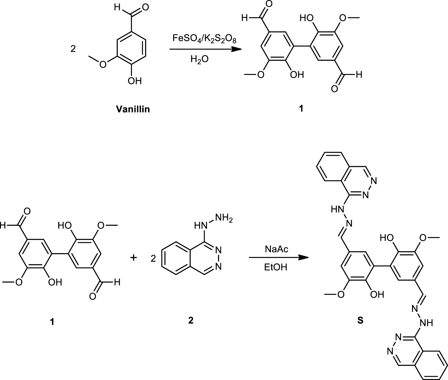
The mixture was heated at 50 °C for 120 h until the reaction was complete as indicated by TLC assay. After cooling at room temperature, the crude product was filtered and washed twice with cold ethanol. Product 1, which had a dark brown color, was obtained after a crystallization process with methanol and dried under vacuum.
For the synthesis of compound S, a suspension of HPT (2) (0.26 g, 1.32 mmol) and sodium acetate (1.85 g, 22.55 mmol) in water (10 mL) was added to a solution of compound 1 (0.20 g, 0.66 mmol) in ethanol (10 mL). The mixture was heated to reflux for four days, and the reaction was monitored by TLC. After cooling to room temperature, the solid product was collected by filtration and washed with water. The final product was obtained after crystallization with 2-propanol and dried under vacuum.
2.3. UV–Vis experiments
2.3.1. Evaluation of sensor selectivity toward cations by UV–Vis spectroscopy
The evaluation of the sensor with different cations were carried out by adding 2.0 mL of sensor solution (10 μM) to 2.0 mL of the cation solutions already described (10 μM). After mixing the solutions for 30 s, the absorbance spectra were recorded from 200 to 600 nm at a scanning speed of 240 nm/min against a blank of distilled water.
2.3.2. Evaluation of complex sensor-Cu2+ stoichiometry
Aqueous solutions of sensor S (1.0 mM) and Cu2+ (1.0 mM) were prepared. Then, both were mixed to generate a series of solutions with Cu2+ mole fractions ranging from 0 to 1, keeping constant the total concentration system. According to this, volumes of 2.0, 1.8, 1.6, 1.4, 1.2, 1.0, 0.8, 0.6, 0.4, 0.2 and 0 mL of the sensing solution were taken and mixed with volumes of 0, 0.2, 0.4, 0.6, 0.8, 1.0, 1.2, 1.4, 1.6, 1.8, 2.0 mL of Cu2+ solution. The total volume was always 2.0 mL. After 30 s of mixing, the absorbance at 420 nm of mixtures were recorded. Absorbances were normalized against solutions prepared by replacing the volume of the cation solution with distilled water.
2.3.3. UV–Vis titration of Cu2+ with S
Titration assays of Cu2+ with S were done by adding 1.0 mL of the sensor solution (100 μM) at 2.0 mL of aqueous solutions of Cu2+ with different concentrations. In these solutions, the final concentration of S was 33 μM, and the concentration range of Cu2+ was from 0 to 133 μM. The absorption spectra of each solution were acquired after 30 s of mixing.
2.4. FTIR experiments
A mixture of 1.0 mL of stock solution (10 mM) of Cu2+ in distilled water together with 1.0 mL of stock solution (10 mM) of sensor S in DMSO/ethanol (v∕v = 2∕8) was prepared. A mixture control of S was prepared using 1.0 mL of distilled water and the same volume of the stock solution of the sensor. Mixtures were heated at 100 °C until complete solvent evaporation. Solid products were diluted with KBr (1 wt%) and pressed into tablets before spectrum acquisition.
2.5. Theoretical modeling
The ground state geometry optimization of sensor S and complex cation sensor with Cu2+ cation were carried out at the DFT level of theory using the CAM-B3LYP correlation function with a 6-31G(d,p) basis set. Frequency calculations allowed us to verify that currently found geometries were minimal. Molecular orbital calculations were performed to characterize the molecular properties. All of these calculations were carried out using Gaussian 09 program package [18].
2.6. Determination of Cu2+ in water samples
Real water samples from the Setubal Lagoon and Colastine River of Santa Fe and two waste water samples were analyzed for Cu2+ determination, previously filtered to remove solid particles in suspension. For the assay, 1.0 mL of the sensor solution (100 μM) was added to 2.0 mL of samples. After mixing the solutions, UV–Vis spectra were obtained.
3. Results and discussion
3.1. Synthetic procedure of sensor
Sensor S has been synthesized following a schematic route depicted in Scheme 1 and described in the experimental section. Characterization of precursor 1 and sensor S are summarized below:
Compound 1: 6,6′-dihydroxy-5,5′-dimethoxy-[1,1′-biphenyl]-3,3′-dicarbaldehyde (3); brown powder; yield 88%; m.p. > 290 °C, 1H NMR (DMSO-d6, 300 MHz): 3.83 (s, 6H, OCH3); 7.36 (d, 2H, CAr–H); 7.32 (d, 2H, CAr–H); 5.21 (s, 2H, CAr–OH); 9.71 (s, 2H, CHO); 13C NMR (DMSO-d6, 300 MHz): 192 (CHO); 158 (C-1); 150 (C-2); 110 (C-3); 128 (C-4); 125 (C-5); 129 (C-6); 56 (CH3). IR (KBr, cm−1): 3264.2 (OH); 1674.2 (C =O); 1587.4 (C =C Arom.); m/z: 302.08; Anal. Calc. for C16H14O6: C, 65.75; H, 4.14; O, 19.17. Found: C, 65.43; H, 4.10; O, 18.97.
Compound S: 3,3′-dimethoxy-5,5′-bis((E)-(2-(phthalazin-1-yl)hydrazono)methyl)-[1,1′-biphenyl]-2,2′-diol; Brown powder; yield 90%; m.p. > 280 °C, 1H NMR (DMSO-d6, 300 MHz): 8.77 (s, 2H, CAr–H); 8.23 (s, 2H, HC =N); 7.95 (m, 4H, CAr–H); 7.88 (m, 4H, CAr–H); 7.47 (s, 2H, CAr–H); 7.58 (s, 2H, CAr–H); 4.03 (s, 2H, NH); 3.41 (s, 6H, OCH3); 13C NMR (DMSO-d6, 300 MHz): 130.7 (C =O); 146.8 HC =N; 111 (C3); 127.8 (C4); 128.3 (C6); 157.6 (C1); 123.7 (C5); 152 (C2); 56,1 (OCH3); IR (KBr, cm−1): 3400 (O–H, N–H); 1630 (C =C); 1580 (C =N); m/z: 586.21; Anal. Calc. for C32H26N8O4: C, 65.52; H, 4.47; N, 19.10; O, 10.91. Found: C, 65.50; H, 4.50; O, 10.87.
3.2. Photochromic properties of sensor
Selectivity is the first parameter that must be evaluated in the development of a new chemosensor [19]. This defines the sensing performance, and in this context describes its ability to identify certain compounds in an unknown mixture [20].
Evaluation of sensor S selectivity with different cations by UV–Vis spectroscopy: (A) UV–Vis absorption spectra of sensor with cations; (B) absorbance at 420 nm of S solutions with different cations.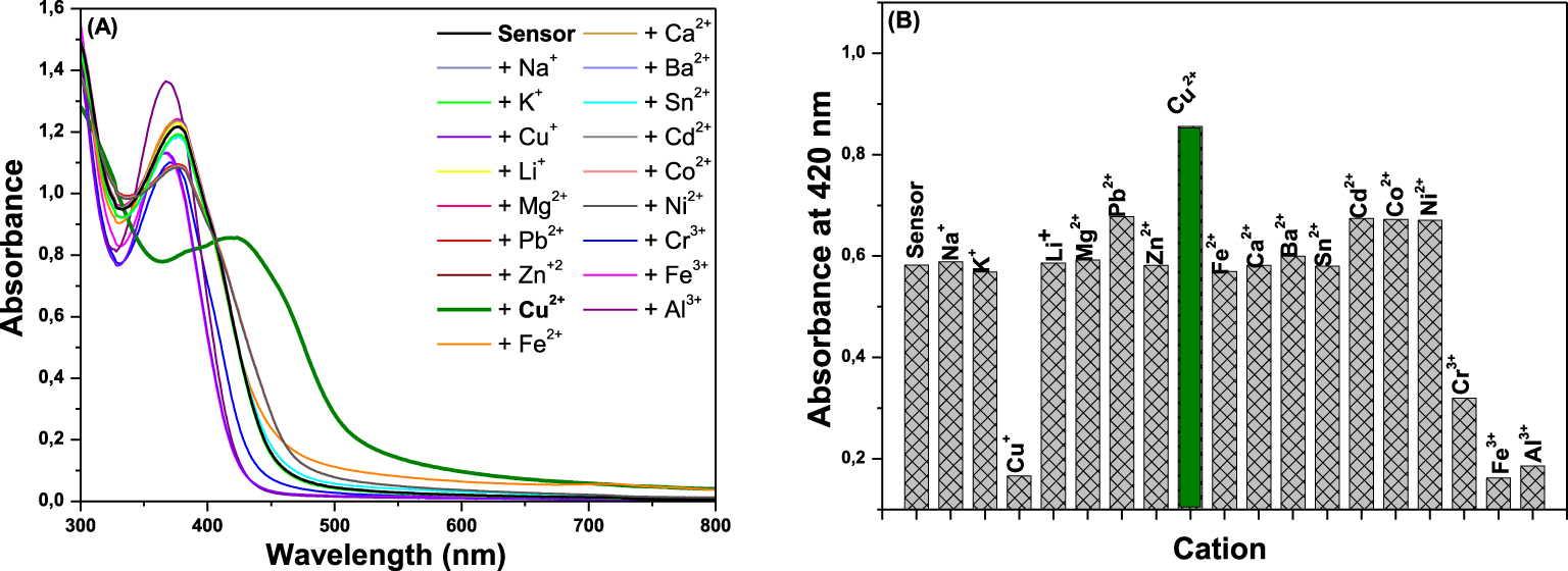
The selectivity of sensor S toward different cations was studied using UV–Vis spectroscopy by analyzing absorption spectra changes of the solution sensor S (10.0 μM) when cation solutions of the same concentration were added separately. In these solutions, the final concentration of S and cations were 5 μM. Spectral changes of S in the presence of different cations are shown in Figure 1A. As can be seen in this figure, the UV–Vis spectrum of sensor S shows a characteristic absorption band at 378 nm. With the addition of cations into the sensing solution, the spectra observed were different. Upon addition of Li+, Na+, Mg2+ and Fe2+ cations in the solution of S, the band at 378 nm increased its intensity, whereas with the addition of K+, Pb2+, Zn2+, Ca2+, Ba2+, Sn2+, Cd2+, and Ni2+ cations into S solution, band intensity at 378 nm decreased. On the other hand, the addition of other cations on sensor solution produced a band shift toward a lower wavelength (hypsochromic shift) together with the increase in the intensity of the band for Al3+ cation and the decrease in the intensity of the band for Cu+, Fe3+, and Cr3+ cations. Particularly, a significant change was observed when Cu2+ cation was added; a new peak appeared at 420 nm for a bathochromic shift indicating that sensor S forms a chromogenic complex with Cu2+.
The absorbance at 420 nm of sensor S in presence of different cations are shown in Figure 1B. As can be seen in this figure, the intensity of sensor S solution at 420 nm increased about 50% after Cu2+ addition, maintaining its maximum value for more than 1 h. These results demonstrated that S presents an excellent selectivity for Cu2+ cation by UV–Vis spectroscopy. The pH of all samples was between 4.0 and 6.5, range in which our analysis method was verified.
3.3. Determination of binding mode between sensor S and Cu2+
Continuing with the evaluation of sensor properties of S with Cu2+, the binding mode between S and Cu2+ was determined according to continuous-variation method. To build Job’s plot, the Cu2+ molar fraction has been variated from 0 to 1 maintaining the total concentration of the solution constant (0.1 mM), and the absorbance value of these solutions has then been reported. The binding stoichiometry of the complex between Cu2+ and S was determined from the Job’s plot and corresponds to the value on the x-axis by the maximum value of absorbance. Figure 2 represents the absorbance variation value at 420 nm versus Cu2+ mole fraction, and the maximum value of absorbance was obtained at a mole fraction of 0.33, indicating a 2:1 stoichiometry for the complex between sensor S and Cu2+.
Job’s plot of sensor S with Cu2+ according to continuous-variation method, indicating 2:1 stoichiometry for S:Cu2+.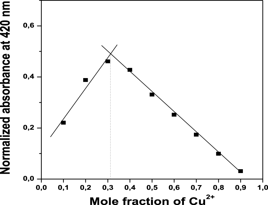
UV–Vis titration with increasing of Cu2+ concentration: (A) spectra of solution S at different Cu2+ concentrations; (B) plot of Ln (A–A0)/(Am–A) as a function of 0.5∗Ln (Cu2+).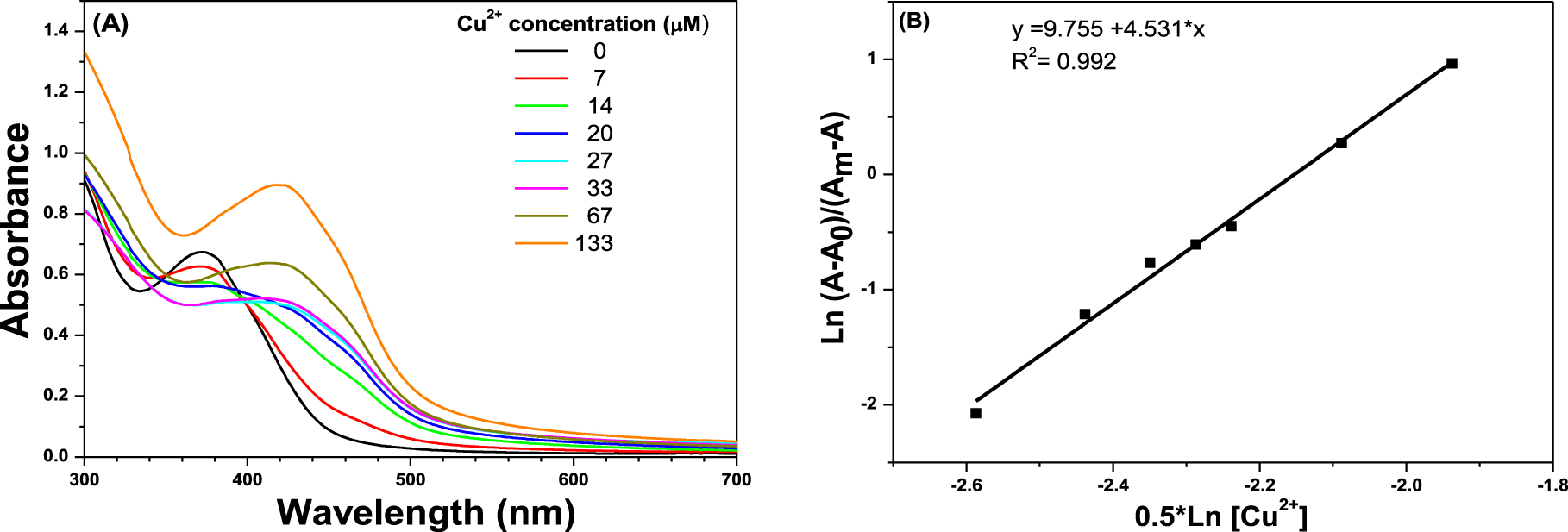
Continuing with the evaluation of binding mode between S and Cu2+, the UV–Vis titration of Cu2+ with sensor S was carried out to determine the binding association constant. The UV–Vis titration was performed by adding Cu2+ solutions from a concentration of 0 to 133 μM into a solution of S (33 μM). Figure 3A shows the absorption spectra of S with increasing Cu2+ concentration. Under experimental conditions, the UV–Vis spectrum of S exhibits an absorption band at 372 nm. Further addition of Cu2+ solution into the S solution resulted in a gradual decrease in the absorbance band at 372 nm (Cu2+ concentration from 0 to 14 μM) associated with the bathochromic shift of the band to higher wavelengths centered at 420 nm (Cu2+ concentration from 20 to 133 μM). The molar extinction coefficient (𝜀) of S–Cu2+ complex at 420 nm was 1.56 × 10⁴ M−1⋅cm−1, two times larger than S coefficient.
Considering a ratio stoichiometry between S and Cu2+ as 1:n, the equilibrium interaction is given by (1):
| (1) |
| (2) |
| (3) |
| (4) |
| (5) |
| (6) |
3.4. Optimization of Cu2+ chemosensing
To optimize the Cu2+ chemosensing conditions of sensor S, the linear range of quantification was evaluated by absorption spectroscopy. It was assumed that the Beer’s law is dependent on the analyte concentration and it is applicable to the quantitative detection of Cu2+.
Linearity study of Cu2+: (A) Evaluation of the linear range of quantification of Cu2+; (B) plot of normalized absorbance at 420 nm as a function of Cu2+ concentration in the linear range.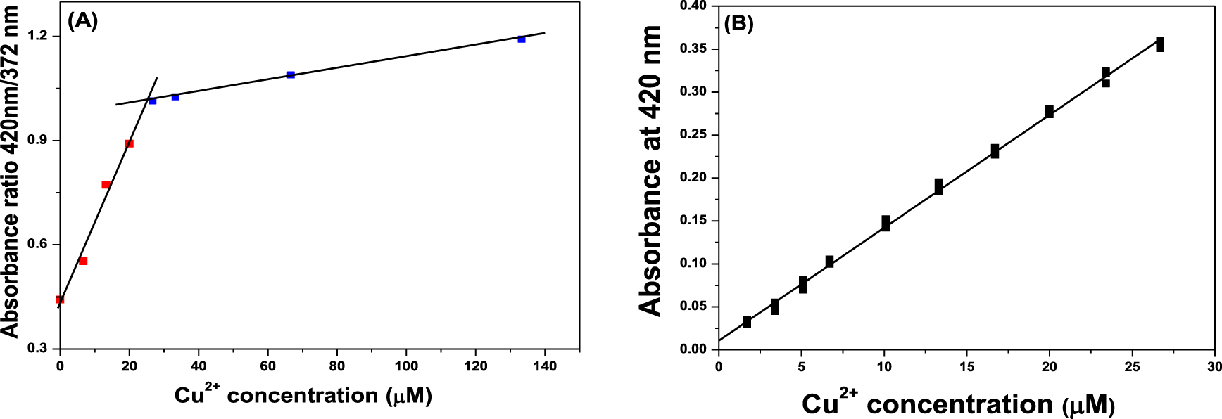
Parameters obtained from calibration assay of Cu2+
| Parameter | Value |
|---|---|
| Slope, a (μM−1) | 0.0132 ± 0.0003 (SD: 0.0001) |
| Intercept, b | 0.0089 ± 0.0037 (SD: 0.0018) |
| Correlation coefficient, R | 0.9986 |
| Analytical sensibility, 𝛾 (μM) | 2.0948 |
| Fexp | 1.000 |
| Ftable (33–2; 33–11; 0.05) | 1.979 |
| Linearity range (μM); (μg⋅L−1) | 5.0–26.7; 315.8–1696.7 |
| Detection limit, DL (μM); (μg⋅L−1) | 1.7; 106.8 |
| Quantification limit, QL (μM); (μg⋅L−1) | 5.0; 315.8 |
SD = standard deviation.
Plotting the absorbance ratio 420 nm/372 nm as a function of the Cu2+ cation concentration from the data obtained at titration experiments, Figure 4A, the linear range curve was constructed. Two UV response regions were identified in Figure 4A, a sensible linear region from 0 to 28 μM Cu2+ corresponding to the linear range quantification of Cu2+, and a second region at Cu2+ concentrations higher than 28 μM of low sensitivity quantification of Cu2+ denominated as a non-linear region.
Considering the linear region of the curve of Figure 4A, a new calibration curve was plotted between absorbance at 420 nm versus concentration of Cu2+ at 11 concentration levels (Figure 4B). Absorbances at 420 nm of standard solutions were normalized against the absorbance of a sensor solution at the same wavelength. The regression data together with the statistical parameters obtained by least-squares fitting of the calibration curve for Cu2+ are summarized in Table 1. High correlation coefficient value (R > 0.99) indicates excellent linearity. The data used in the calibration was analyzed using lack of fit test to determine whether the linear model is suitable to describe the observed data, verified that the experimental data fit with the linear law.
The data obtained from the linearity study was used to determine the detection limit (DL) and quantification limit (QL) using the expression according to recommendation in literature [21], employing (7) and (8), respectively:
| (7) |
| (8) |
Results from accuracy and precision assays
| Accuracy evaluation | Precision evaluation | |||||||
|---|---|---|---|---|---|---|---|---|
| Sample | Cu2+ concentration (μM) | R (%) | n | Cu2+ concentration (μM) | ||||
| Nominal | Found | Sample 1 | Sample 2 | Sample 3 | ||||
| 1 | 2.30 | 2.26 (0.05) | 98.1 | 1 | 3.15 | 5.22 | 11.41 | |
| 2 | 4.10 | 4.09 (0.04) | 99.8 | 2 | 3.12 | 5.23 | 11.42 | |
| 3 | 7.50 | 7.44 (0.07) | 99.2 | 3 | 3.15 | 5.20 | 11.40 | |
| 4 | 12.00 | 12.03 (0.11) | 100.2 | 4 | 3.20 | 5.25 | 11.43 | |
| 5 | 17.40 | 17.39 (0.08) | 99.9 | 5 | 3.12 | 5.20 | 11.39 | |
| X | 3.15 | 5.22 | 11.41 | |||||
| SD | 0.03 | 0.02 | 0.02 | |||||
| RSD (%) | 0.95 | 0.38 | 0.17 | |||||
X = average; SD = standard deviation; RSD = relative standard deviation.
The preferential selectivity of sensor S toward Cu2+ in the presence of other cations was also analyzed.
The possible interference of other cations was evaluated by adding 33 μM of S to cations solutions (66 μM) in the presence and absence of 33 μM of Cu2+. After mixing, the absorbance of each solution was recorded at 420 nm and normalized with a blank sample. The results are shown in Figure 5, and they confirmed that the selective quantification and detection of Cu2+ was not influenced by the presence of common cations. No significant absorbance variation was observed during sample comparison between Cu2+ and other cations.
Cation selectivity profiles of sensor S toward Cu2+ when other cations are present.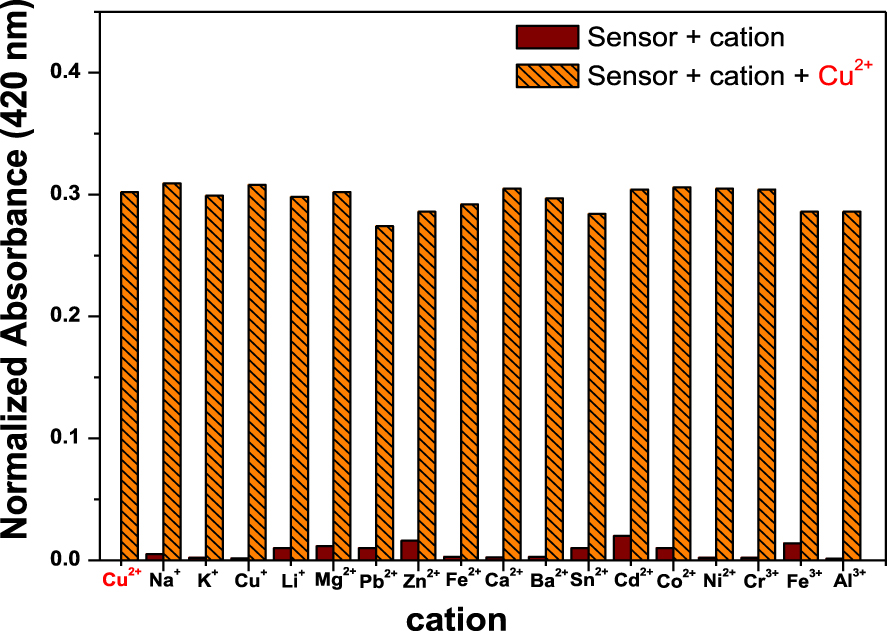
The accuracy of the analytical method was evaluated by analyzing the recovery (R) of five samples containing known Cu2+ amounts. Recovery values in the range of 90–107% are considered as the criterion for a suitable recovery [19]. Table 2 shows the results and, as it can be noticed, recovery percentages near 100% for all the samples were obtained. Although the concentration of sample 1 is less than QL, the concentration found and the recovery were adequate, indicating the excellent performance of the analytical method. These recovery values were tested statistically by the averaged recovery method, demonstrating that the method is accurate.
In order to further study the precision of the analytical method, three samples were analyzed five times. Data of standard deviations and relative standard deviations (RSD) for Cu2+ determination in Table 2 showed a good repeatability of the results. The RSD values were in all cases lower than 1%.
According to these results it is possible to conclude that the proposed analytical method is selective, linear, precise and accurate for the qualitative and quantitative determination of Cu2+ by UV–Vis spectroscopy.
3.5. Molecular modeling of the complex sensor-Cu2+
Theoretical calculations based on DFT were performed to understand the binding mode of Cu2+ cation with the sensor S.
Optimized structures of Sensor S and Sensor-Cu2+ complex.
The optimized structures of sensor S and sensor-Cu2+ complex are shown in Figure 6. From these structures, it can be seen that nitrogen atoms of hydralazine moieties are participating in the complex formation. The N–Cu2+ bonds range from 1.91 to 2.12 Å.
Considering a ratio stoichiometry between S and Cu2+ as 2:1, the binding energy (BE) was estimated by the (9):
| (9) |
The complex formation between Cu2+ and S involves charge transfer, which occurs between the highest occupied molecular orbital (HOMO) and the lowest unoccupied molecular orbital (LUMO). The distribution of HOMO–LUMO orbitals of S and S2–Cu2+ complex and the energy difference (gap energy) between those orbitals are shown in Figure 7.
HOMO–LUMO orbitals distribution of Sensor S and Sensor-Cu2+ complex.
In the presence of Cu2+ ion, upon Cu2+ binding with nitrogen atoms of phthalazine units, the energy levels of both HOMO and LUMO are lower than those of free S. Also, the decrease of energy in the LUMO is more significant than for the HOMO, indicating that the LUMO is more stabilized.
The decrease in energy gap between S and S2Cu2+ is in agreement with the experimental bathochromic changes in spectra of S, upon complexing with Cu2+.
3.6. Theoretical–experimental evaluation of the complex sensor Cu2+
In order to evaluate the functional groups involved in S2–Cu2+ complex formation, FTIR spectra of S and S2–Cu2+ were recorded, and are shown in Figure 8.
FTIR spectra of S Sensor and Sensor-Cu2+ complex. (A) Experimental; (B) Theoretical.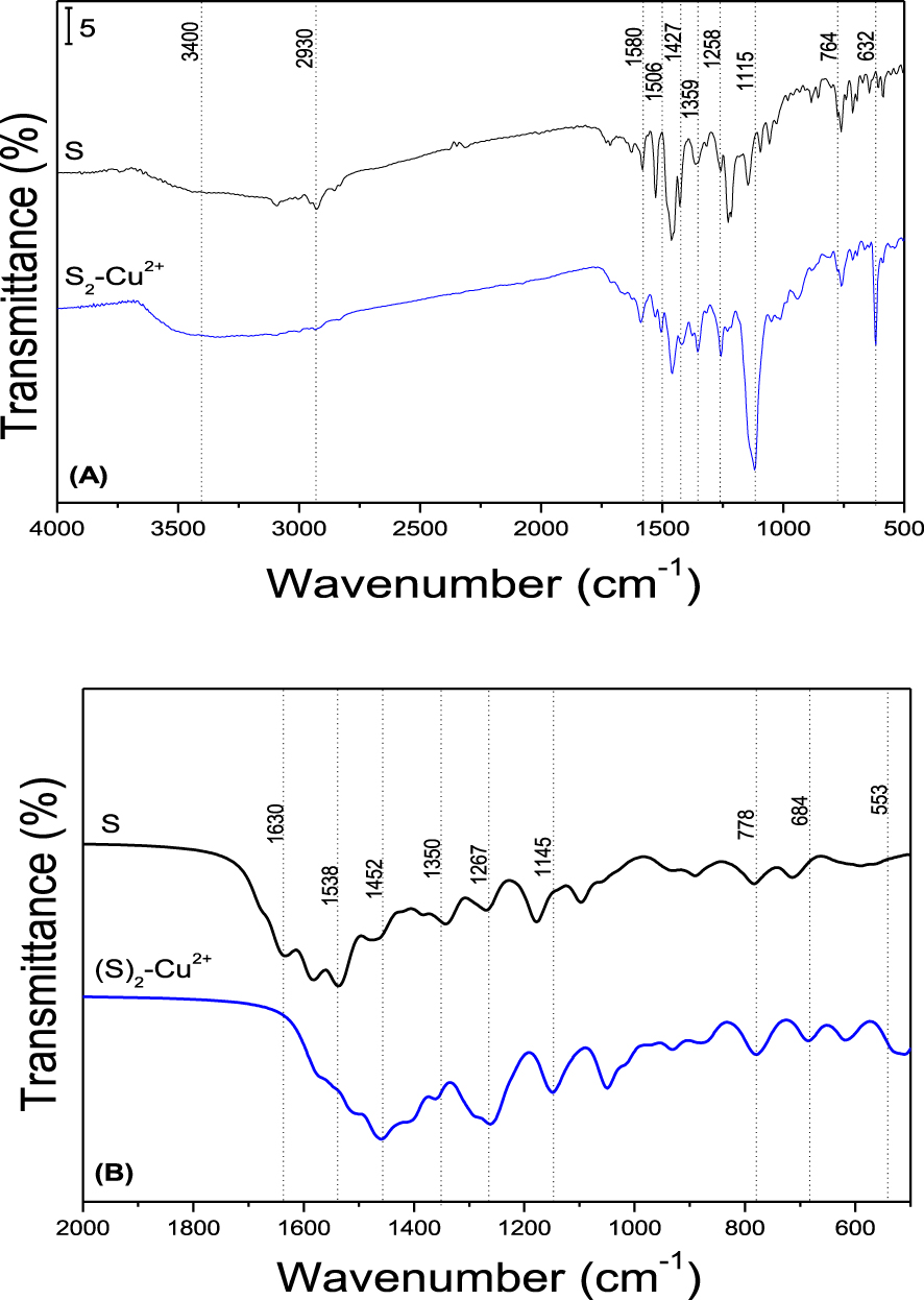
For the spectrum of ligand S, (Figure 8A, black line spectrum), it is possible to identify two main regions: 3600–2700 cm−1 and 1600–1000 cm−1. The region from 3600–2700 cm−1 shows a broad band, assigned to O–H and N–H stretching, while the bands between 3100–2800 cm−1 are assigned to C–H stretching vibrations [23, 24, 25].
In the region from 1600–1000 cm−1 the main identification bands are observed. The vibrations at 1580 cm−1 and 1530 cm−1 are assigned to C =N and C–N stretching, respectively [24, 25, 26]. The bands at 1630 cm−1 and 1427 cm−1 correspond to C =C and C–C stretching vibrations, respectively, and the band at 1228 cm−1 is assigned to C =C stretching vibrations present in aromatic systems [24, 25, 26, 27]. The bands observed at 1364, 1330 and 1263 cm−1 are assigned to N–N, N–N–H and C–N stretching vibrations respectively; while the bands at 1142, 764 and 640 cm−1 correspond to C–C =C, C–N–N and C–C =N bending modes [26].
When the FTIR spectrum of S2–Cu2+ was analyzed, (Figure 8A, blue line spectrum) the main assignations observed in S are identified, with slight differences in intensity and positions. It is observed that the stretching band between 3600–3200 cm−1 due to O–H and N–H groups has increased its intensity, which is attributed to S2–Cu2+ complex association to water molecules through hydrogen bonds [27]. In the region between 1600–1000 cm−1, an intensity increase is observed followed by a shift to lower frequencies for C–C =N bending, and N–N, C–N stretching, at 623, 1359 and 1258 cm−1 respectively. Also, an intensity decrease is observed at 1506, 1464, 1452 and 1222 cm−1 assigned to C–C and C =C stretching vibrations. The band at 1115 cm−1 is attributed to counter ion present in the sample [24, 25, 26, 27], while the band at 539 cm−1 corresponds to N–Cu stretching mode in the complex [28, 29]. These results suggest that phthalazine nitrogen atoms present in S ligands would participate in Cu2+ complex formation.
In order to validate these experimental results, theoretical spectra for S and S2–Cu2+ were calculated.
Results obtained from Cu2+ determination in real water samples
| Quantification evaluation | Recovery evaluation | ||||||||
|---|---|---|---|---|---|---|---|---|---|
| Cu2+ concentration (μg∕L) | Cu2+ concentration (μg∕L) | Recovery (%) | |||||||
| Sample | ICP-MS | L | Entry | Initial | Added | Theoretical | Found | ||
| Colastiné river | 40 | 35 | 1 | 450 | 0 | 450 | 438 | 97 | |
| Setubal lake | 435 | 467 | 2 | 450 | 600 | 1050 | 1062 | 101 | |
| Tap water | 272 | 297 | 3 | 1270 | 0 | 1270 | 1263 | 99 | |
| Waste water 1 | 2115 | 2090 | 4 | 1270 | 480 | 1750 | 1725 | 99 | |
| Waste water 2 | 1695 | 1680 | 5 | 1270 | 820 | 2090 | 2140 | 102 | |
Mainly, when S and S2–Cu2+ spectra are compared in the region between 3600–2900 cm−1, the O–H, N–H and C–H stretching vibrations are observed (region not shown in Figure 8B) with a slight increase in intensity of these bands in complex S2–Cu2+ spectrum. Significant changes are detected in the region between 2000–500 cm−1 (Figure 8B).
Just as observed when experimental FTIR spectra were compared, the main band changes correspond to N–N, C–N stretching and C–C =N bending.
An increase in intensity and a shift to lower frequencies is observed on comparing S2–Cu2+ spectrum against free S. The band at 706 cm−1 in free S FTIR spectrum, assigned to C–C =N bending, is present in S2–Cu2+ spectrum at 684 cm−1; while the bands at 1385 and 1267 cm−1 in S spectrum, assigned to N–N and C–N stretching, are identified in S2–Cu2+ spectrum at 1360 and 1260 cm−1 respectively.
These spectra changes are accompanied by a shift to lower frequencies for C–C =C, N–N–H and C–N–N bending signals in S at 1178 cm−1, 1354 cm−1 and 786 cm−1, respectively, in the complex at 1145 cm−1, 1350 cm−1 and 778 cm−1, respectively.
Also, the interaction of Cu2+ and ligand molecules is done through phthalazine nitrogens, which is concluded with the band at 553 cm−1 assigned to N–Cu stretching in the S2–Cu2+ FTIR spectrum. In addition to this, in free S spectrum an increase intensity is observed for C =N and C–N stretching, positioned at 1538 cm−1 and 1455 cm−1, respectively; along with intensity decrease for C =C and C–H stretching, present in the region between 1515–1490 cm−1 [28, 29]. This allows us to validate the observed FTIR results for S and complex, verifying the interaction of Cu2+ in the S2–Cu2+ complex.
3.7. Determination of Cu2+ in real water samples
To evaluate the practical application of the validated method, different real water samples were analyzed. These samples were centrifuged, filtered and analyzed by Inductively Coupled Plasma Mass Spectrometry (ICP-MS) and by our developed method (L).
The pH of all samples was between 4.0 and 6.5, which corresponds to the pH range in which our analysis method was verified. Results are presented in Table 3 (left) showing a good correlation between both techniques, indicating that our method would be suitable to routinely analyze the Cu2+ content in real samples.
Furthermore, in order to analyze the method performance in real samples, two real water samples whose content was previously determined by ICP-MS, were enriched by adding known amounts of Cu2+. Subsequently, the samples were analyzed by our method and, based on the theoretical and experimental concentrations obtained, the Cu2+ recovery was evaluated. The results (Table 3, right) showed a good correlation between found and theoretical concentrations, showing an adequate method performance to determine Cu2+ cation concentrations in real water samples.
4. Conclusions
In summary, a new selective colorimetric chemosensor was synthesized and applied for Cu2+ detection in aqueous samples. The sensor S was obtained through a simple synthetic pathway and it was obtained with good yield. The sensor has shown selectivity and sensitivity toward Cu2+, the limit of detection for this cation being 1.7 μM. The proposed analytical method is precise and accurate for Cu2+ determination and it was successfully applied to real water samples, the results being in agreement to those obtained by more sophisticated techniques.
Acknowledgment
This work was supported by the Universidad Nacional del Litoral (Capital Semilla 2019 Grant), Santa Fe, Argentina.
Supplementary data
Supporting information for this article is available on the journal’s website under https://doi.org/10.5802/crchim.131 or from the author.