Fracture roughness and thermal exchange: A case study at Soultz-sous-Forêts

Amélie Neuville; Renaud Toussaint; Jean Schmittbuhl

doi:10.1016/j.crte.2009.03.006

Surface geosciences (Hydrology–hydrogeology)

Fracture roughness and thermal exchange: A case study at Soultz-sous-Forêts
[Rugosité de fracture et échange thermique : étude de cas à Soultz-sous-Forêts]

Présenté par : Written on invitation of the Editorial Board

Amélie Neuville ^1,² ; Renaud Toussaint ^1,² ; Jean Schmittbuhl ^1,²

¹ UMR CNRS 7516, institut de physique du globe de Strasbourg, 5, rue Descartes, 67084 Strasbourg cedex, France
² EOST, université de Strasbourg, Strasbourg, France

Comptes Rendus. Géoscience, Volume 342 (2010) no. 7-8, pp. 616-625.

Résumés

Anglais
Français

Heat exchange during laminar flow in an open fracture is studied numerically on the basis of the Stokes equation in the limit of hydrothermal lubrication. We examine the influence of fracture roughness on hydraulic permeability and heat flux through the fracture sides when a cold fluid is injected into a homogeneous hot host rock. Spatial temperature fluctuations inside the fluid are studied assuming the temperature of the rock to be constant and the fracture aperture to be self-affine. An application to the case study at the deep geothermal reservoir of Soultz-sous-Forêts, France, is presented. Finally, a thermal model based on sparse spatial information of the geometrical aperture is successfully proposed to reproduce the response of the fracture.

L’échange de chaleur en régime laminaire est étudié numériquement dans une fracture ouverte sur la base de l’équation de Stokes, dans la limite de l’hypothèse de lubrification hydrothermique. Nous observons l’influence de la rugosité sur la perméabilité hydraulique, ainsi que sur le flux de chaleur à travers les parois de la fracture, quand un fluide froid est injecté dans une roche mère ayant une température chaude homogène. Les fluctuations de la température du fluide sont étudiées en supposant que la température de la roche est constante et la fracture auto-affine. Une application au cas d’étude du réservoir de géothermie profonde à Soultz-sous-Forêts, France, est présentée. Finalement, nous proposons un modèle thermique basé sur la connaissance spatiale réduite de l’ouverture géométrique, qui reproduit bien la réponse de la fracture.

Métadonnées

Reçu le : 2008-11-11
Accepté le : 2009-03-17
Publié le : 2009-06-10

DOI : 10.1016/j.crte.2009.03.006

Keywords: Fracture, Roughness, Lubrication, Heat exchange, Soultz-sous-Forêts, France
Mot clés : Fracture, Rugosité, Lubrification, Échange de chaleur, Soultz-sous-Forêts, France

Affiliations des auteurs :

Amélie Neuville ^{1, 2} ; Renaud Toussaint ^{1, 2} ; Jean Schmittbuhl ^{1, 2}

¹ UMR CNRS 7516, institut de physique du globe de Strasbourg, 5, rue Descartes, 67084 Strasbourg cedex, France
² EOST, université de Strasbourg, Strasbourg, France

@article{CRGEOS_2010__342_7-8_616_0,
     author = {Am\'elie Neuville and Renaud Toussaint and Jean Schmittbuhl},
     title = {Fracture roughness and thermal exchange: {A} case study at {Soultz-sous-For\^ets}},
     journal = {Comptes Rendus. G\'eoscience},
     pages = {616--625},
     publisher = {Elsevier},
     volume = {342},
     number = {7-8},
     year = {2010},
     doi = {10.1016/j.crte.2009.03.006},
     language = {en},
}

TY  - JOUR
AU  - Amélie Neuville
AU  - Renaud Toussaint
AU  - Jean Schmittbuhl
TI  - Fracture roughness and thermal exchange: A case study at Soultz-sous-Forêts
JO  - Comptes Rendus. Géoscience
PY  - 2010
SP  - 616
EP  - 625
VL  - 342
IS  - 7-8
PB  - Elsevier
DO  - 10.1016/j.crte.2009.03.006
LA  - en
ID  - CRGEOS_2010__342_7-8_616_0
ER  -

%0 Journal Article
%A Amélie Neuville
%A Renaud Toussaint
%A Jean Schmittbuhl
%T Fracture roughness and thermal exchange: A case study at Soultz-sous-Forêts
%J Comptes Rendus. Géoscience
%D 2010
%P 616-625
%V 342
%N 7-8
%I Elsevier
%R 10.1016/j.crte.2009.03.006
%G en
%F CRGEOS_2010__342_7-8_616_0

Amélie Neuville; Renaud Toussaint; Jean Schmittbuhl. Fracture roughness and thermal exchange: A case study at Soultz-sous-Forêts. Comptes Rendus. Géoscience, Volume 342 (2010) no. 7-8, pp. 616-625. doi : 10.1016/j.crte.2009.03.006. https://comptes-rendus.academie-sciences.fr/geoscience/articles/10.1016/j.crte.2009.03.006/

Version originale du texte intégral

1 Introduction

Modeling of the fluid transport in low permeable crustal rocks is of central importance for many applications (Neuman, 2005). Among them is the monitoring of the geothermal circulation in the project of Soultz-sous-Forêts, France, (Bachler et al., 2003) where the heat exchange especially occurs through open fractures in granite (Gérard et al., 2006).

Numerous hydrothermal models have already been proposed. For simple geometries, some analytical solutions are known: e.g., the cases of parallel plates (Turcotte and Schubert, 2002) or flat cylinders (Heuer et al., 1991). More complex models exist as well like the models of three-dimensional (3D) networks of fractures reproducing geological observations and possibly completed with stochastical distributions of fractures (e.g. in Soultz-sous-Forêts, France, (Gentier, 2005; Rachez et al., 2007) or in Rosemanowes, UK (Kolditz and Clauser, 1998)). Nevertheless, the geometry of each fracture is generally simple. Kolditz and Clauser (1998) have however suspected that differences between heat models and field observations could be due to channeling induced by the fracture roughness or the fracture network. Channeling of the fluid flow owing to fracture roughness has indeed already been experimentally observed and studied (Méheust and Schmittbuhl, 2000; Plouraboué et al., 2000; Schmittbuhl et al., 2008; Tsang and Tsang, 1998).

Here, we limit our study to the fracture scale and we will show only one example of thermal behavior, among other simulations we completed (Neuville et al., submitted). The specificity of our hydrothermal model is to take into account the different scale fluctuations of the fracture morphology. We aim at bringing out the main parameters, which control the hydraulic and thermal behavior of a complex rough fracture. The perspective is to propose a small set of effective parameters that could be introduced within simplified elements for an upscaled network model.

We first describe our geometrical model of the fracture aperture thanks to self-affine apertures. Then, using lubrication approximations, we obtain the bidimensional (2D) pressure and thermal equations when a cold fluid is injected through the fracture in a stationary regime. The temperature within the surrounding rock is supposed to be hot and constant in time and space. The fluid density is also supposed to be constant.

We apply our numerical model to the case study at Soultz-sous-Forêts and we show for this case an example of the computed hydraulic and thermal behavior. Finally, we aim at bringing out what is the minimal geometrical information needed to get the dominant behavior of the hydraulic and thermal fields. This last approach is based on spatial low pass Fourier filtering of the geometrical aperture field.

2 Modeling

2.1 Roughness of the fracture aperture

We consider that the mean fracture plane is described by the $(\hat{x}, \hat{z})$ coordinates and the perpendicular direction is $\hat{y}$ (Fig. 1) – where the hat notation refers to unit vectors along the (x,y,z) axis. It has been shown that a possible geometrical model of natural rough fractures consists in self-affine surfaces. A surface described by a function y = f(x,z) is self-affine if it is statistically invariant under the scaling transformation x → λx, z → λz and y → λ^ζy, where ζ is called the roughness exponent or Hurst exponent. Such surfaces are therefore statistically invariant upon an isotropic scaling within their mean plane while along the perpendicular direction, the scaling is anisotropic (e.g. Brown and Scholz, 1985; Cox and Wang, 1993; Power et al., 1987; Schmittbuhl et al., 1993, 1995). Most fracture surfaces in heterogeneous material exhibit a Hurst exponent equal to ζ = 0.8 (Bouchaud, 1997; Santucci et al., 2007; Schmittbuhl et al., 1993, 1995). Sandstone fractures, however, show ζ = 0.5 (Boffa et al., 1998; Méheust, 2002).

Fig. 1
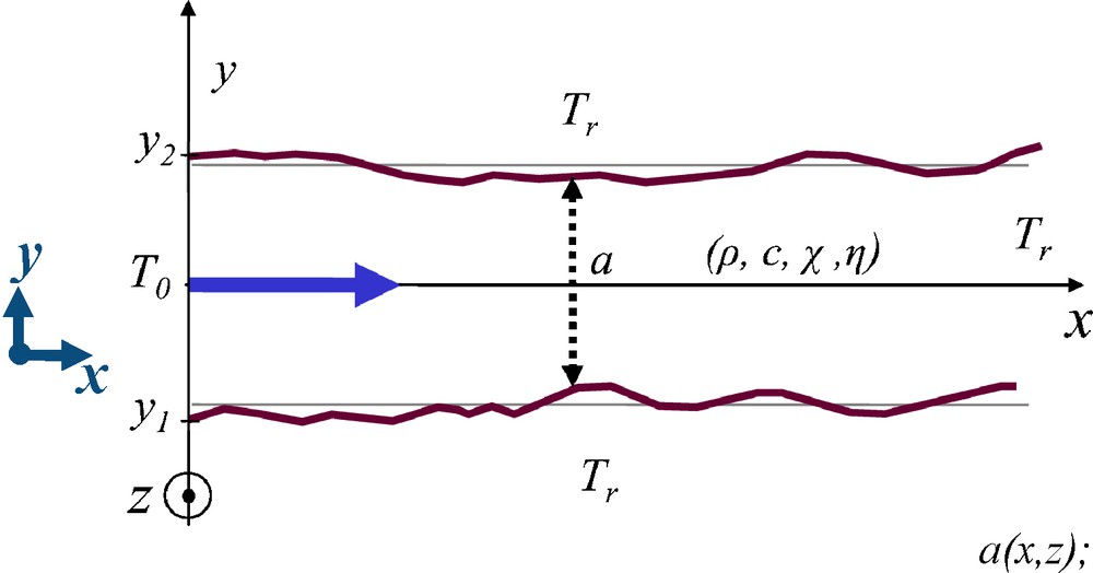
Schematic fracture with variable aperture a(x,z); ρ, c, χ, η are respectively the following fluid properties: density, heat capacity, thermal diffusivity and dynamic viscosity.
Schéma de fracture ayant une ouverture variable a(x,z); ρ, c, χ, η sont les propriétés respectives suivantes du fluide : densité, capacité thermique, diffusivité thermique et viscosité dynamique.

It is important to note that a self-affine surface having a roughness exponent smaller than one is asymptotically flat at large scales (Roux et al., 1993). Accordingly, the self-affine topography can be seen as a perturbation of a flat interface. When the lubrication approximation (Pinkus and Sternlicht, 1961) holds, in particular with smooth enough self-affine perturbations or highly viscous fluid, only the local aperture controls the flow and not the local slope of the fracture. The accuracy of the lubrication approximation, compared to the full Navier-Stokes resolution, was studied in Al-Yaarubi et al. (2005). Under this assumption, the only required geometrical input is the aperture field (also called the geometrical aperture); there is no need to know the geometry of each facing fracture surfaces. The aperture between two uncorrelated self-affine fracture surfaces having the same roughness exponent is as well self-affine (Méheust and Schmittbuhl, 2003). Thus, we generate the numerical apertures by using self-affine functions.

Several independent self-affine aperture morphologies can be generated with the same roughness exponent chosen equal to ζ = 0.8. They exhibit various morphology patterns according to the chosen seed of the random generator (Méheust, 2002). The mean geometrical aperture A and the root-mean square deviation σ (RMS) of an aperture a(x,z) are defined as

A = \frac{\iint a d x d z}{l_{x} \cdot l_{z}} and

(1)

σ^{2} = \frac{\iint a^{2} d x d z}{l_{x} \cdot l_{z}} - A^{2}

(2)

with l_x the length and l_z the width of the fracture. To keep the boundary geometry of the domain as simple as possible, we do not allow any contact area (i.e. no local aperture equal to zero). This is obtained by considering a large enough aperture average to get strictly positive aperture fields.

It has to be noted that our hydrothermal model can be applied to other geometrical models (i.e. different from a self-affine model), which might be more relevant depending on the geological context.

2.2 Physics of hydraulic flow

The hydraulic flow is obtained under the same hypotheses and solved in the same way as in Méheust and Schmittbuhl (2001). We use finite differences, and the system of linear equations is inverted using an iterative biconjugate gradient method (Press et al., 1992).

We impose a pressure drop across the system and study the steady state flow of a Newtonian fluid at low Reynolds number, so that the viscous term dominates the inertial one in the Navier-Stokes equation (Batchelor, 2002; Stokes, 1846):

\vec{\nabla} P = η Δ {\vec{u}}^{3 D}

(3)

where η is the dynamic viscosity, u^3D the velocity of the fluid and P is the pressure deviation from the hydrostatic profile (or the hydraulic head equal to the pressure corrected by the gravity effect). To be in the framework of the lubrication approximation (Pinkus and Sternlicht, 1961), we consider fractures with constant enough apertures together with a small Reynolds number. In doing so, the velocity vector of the fluid flow has negligible components normal to the mean fracture plane. We consider that the macroscopic pressure gradient is imposed along

\hat{x}

;

\hat{z}

is therefore perpendicular to the mean flow direction. Accordingly, the fluid velocity follows a parabolic law (e.g. Iwai, 1976) (Fig. 2):

{\vec{u}}^{3 D} (x, y, z) = \frac{{\vec{\nabla}}_{2} P}{2 η} (y - y_{1}) (y - y_{2})

(4)

where y₁ and y₂ are the local fracture sides coordinates and

{\vec{\nabla}}_{2}

is the gradient operator in the fracture plane. The hydraulic flow through the fracture aperture follows a cubic law:

\vec{q} (x, z) = \int_{a} {\vec{u}}^{3 D} (x, y, z) d y = - \frac{a^{3}}{12 η} {\vec{\nabla}}_{2} P

(5)

Fig. 2
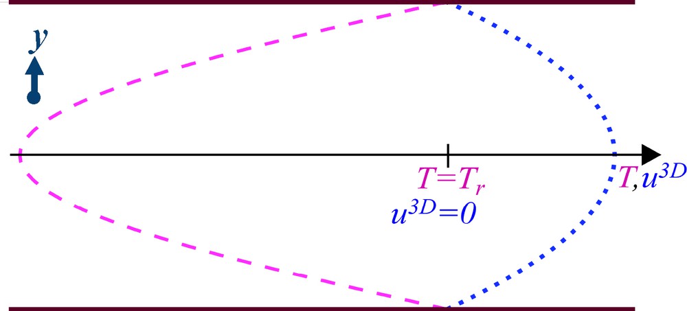
Local velocity quadratic profile (dotted line) and temperature quartic profile (dashed line) inside a fracture across the aperture at the mesh scale. Along the fracture sides, u^3D = 0 and T = T_r, and the roots of the polynoms given by Eqs. (4) and (8) are respected.
Profil local parabolique de vitesse (ligne pointillée) et profil local quartique de température (ligne tiretée) dans la fracture, à travers l’ouverture. Le long des bords, u^3D = 0 et T = T_r et les racines des polynômes donnés par les Éqs. (4) et (8) sont respectées.

and the bidimensional (2D) velocity $\vec{u}$ is defined from the average of the velocity ${\vec{u}}^{3 D}$ over the aperture with

\vec{u} (x, z) = \frac{1}{a (x, z)} \int_{a} {\vec{u}}^{3 D} (x, y, z) d y = - \frac{a^{2}}{12 η} {\vec{\nabla}}_{2} P

(6)

Furthermore, considering the fluid to be incompressible, the Reynolds equation is obtained: ${\vec{\nabla}}_{2} (a^{3} {\vec{\nabla}}_{2} P) = 0$ . As boundary conditions of this equation, we impose the pressure at the inlet and outlet of the fracture (if x = 0, P = P₀ and if x = l_x, P = P_lx, with P₀ > P_lx) and consider impermeable sides at z = 0 and z = l_z.

2.3 Physics of thermal exchange

On the basis of a classical description (e.g. Ge, 1998; Turcotte and Schubert, 2002), we aim at modeling the fluid temperature when cold water is permanently injected at the inlet of a hot fracture at temperature T₀. As the conduction inside the rock is not taken into account (hypothesis of infinite thermal conduction inside the rock), the fracture sides are supposed to be permanently hot at the fixed temperature T_r. This hypothesis should hold for moderate time scales (e.g. minutes), after the fluid injection has stabilized, and before the rock temperature has significantly changed, or alternatively once the whole temperature bedrock is stabilized (which depends on the boundary condition of the entire region). For time scales implying evolution of the rock temperature, our model should be coupled to a model of the rock temperature evolution.

The fluid temperature is controlled by the balance between thermal convection and conduction inside the fluid, which reads (Landau and Lifchitz, 1994): ${\vec{u}}^{3 D} \cdot \vec{\nabla} T = χ Δ T$ where χ is the thermal diffusivity of the fluid and T the fluid temperature. We extend the local lubrication approximation by considering that the slopes of the fracture morphology are small enough to limit the conduction only along the y-axis. We suppose that the leading terms are the conduction along the y-axis and the in-plane convection (since there is no fluid velocity component along $\hat{y}$ ). Indeed, the off-plane free convection has been shown to be negligible (its magnitude is of the order of km/year (Bataillé et al., 2006)). So, the previous equation reduces to:

\frac{\partial^{2} T}{\partial y^{2}} = \frac{{\vec{u}}_{x}^{3 D}}{χ} \frac{\partial T}{\partial x} + \frac{{\vec{u}}_{z}^{3 D}}{χ} \frac{\partial T}{\partial z}

(7)

where

{\vec{u}}_{x}^{3 D}

{\vec{u}}_{z}^{3 D}

are the in-plane components of the fluid velocity. The fluid is supposed to be at rock temperature along the fracture sides, and sufficiently far from the inlet. When we integrate Eq. (7) along the fracture aperture, we assume that β = q_x(∂T/∂x)+q_z(∂T/∂x) is independent of y, where q_x and q_z are the in-plane component of

\vec{q}

defined in Eq. (5). Accordingly, we find that the temperature solution has a quartic profile (Fig. 2) along the fracture aperture:¹

T = - \frac{β}{2 a^{3} χ} (y - y_{1}) (y - y_{2}) (y - \sqrt{5} y_{1}) (y - \sqrt{5} y_{2}) + T_{r}

(8)

where y₁ and y₂ are the local fracture sides coordinates.

Similarly to what is done for the hydraulic flow, we solve the thermal equation by integrating it along the fracture aperture (following the lubrication approximation extended to the thermal field). In particular, when doing the balance of the energy fluxes, we express the advected free energy flux as $ρ c \int_{a} u^{3 D} (x, y, z) [T (x, y, z) - T_{0}] d y$ . Accordingly, we introduce:

\bar{T} (x, z) = \frac{\int_{a} u^{3 D} (x, y, z) T (x, y, z) d y}{\int_{a} u^{3 D} (x, y, z) d y}

(9)

which is an average of the temperature profile weighted by the local norm of velocity. We also use the Nusselt number Nu = φ_r/φ_ref which compares the efficiency of the heat flow along the fracture boundaries:

φ_{r} = \mp χ ρ c {\frac{\partial T}{\partial y}|}_{y = y_{1}, y_{2}}

(10)

to the mesoscopic heat flow at the fracture aperture scale without convection:

φ_{r e f} = χ ρ c (T_{r} - \bar{T}) / a

. Using the polynomial expression of T (in Eq. (8) and the definition of

\bar{T}

, we get

β = 140 χ (T_{r} - \bar{T}) / (17 a)

and Nu = 70/17. Eq. (7) leads then to:

\vec{q} \cdot {\vec{\nabla}}_{2} \bar{T} + 2 \frac{χ}{a} N u (\bar{T} - T_{r}) = 0,

(11)

Boundary conditions are: $\bar{T} (0, z) = T_{0}$ at the inlet and $\bar{T} (l_{x}, z) = T_{r}$ at the outlet (with l_x large enough). Any boundary condition for the temperature along z = 0 or z = l_z can be used as the hydraulic flow $\vec{q}$ is null there.

We discretize this equation by using a first order finite difference scheme and finally get $\bar{T}$ by inverting the system using a biconjugated gradient method (Press et al., 1992).

It is finally possible to get the three-dimensional temperature field T anywhere within the fluid by using the previous β expression and the quartic profile (Eq. (8). Fig. 3 illustrates an example of temperature field at a given z = z₀, T(x,y,z = z₀), obtained in that way from a given bidimensional field $\bar{T}$ . Along any given cut at x = x₀, the temperature (represented by the color scale) follows a quartic law (Fig. 2). The boundaries between the colors are isotherms.

Fig. 3
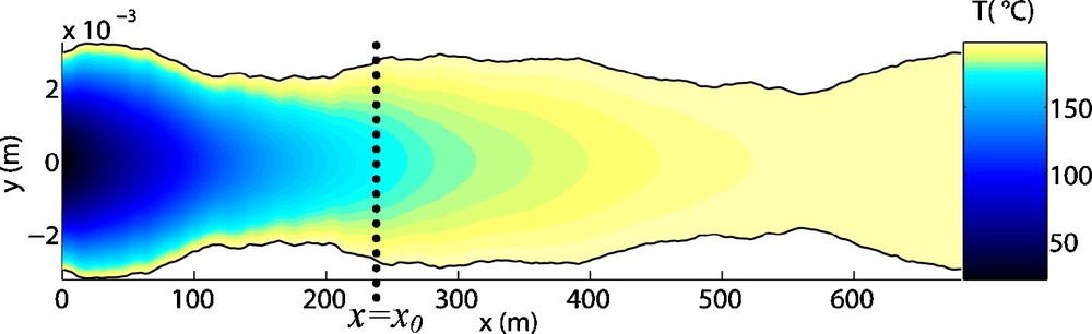
Example of temperature T(x,y,z = z₀) inside a variable aperture between ±a(x,y,z = z₀)/2, computed from $\bar{T}$ shown in Fig. 7, at z = 700 m. The color scale is linear.
Exemple de température T(x,y,z = z₀) à travers l’ouverture variable, entre ±a(x,y,z = z₀)/2, calculé d’après $\bar{T}$ illustré Fig. 7, en z = 700 m. L’échelle de couleur est linéaire.

2.4 Definition of characteristic quantities describing the computed hydraulic and thermal fields

2.4.1 Comparison to modeling without roughness

If we consider a fracture modeled by two parallel plates separated by a constant aperture A, then the gradient of pressure is constant all along the fracture as well as the hydraulic flow which is equal to:

{\vec{q}}_{/ /} = - \frac{Δ P}{l_{x}} \frac{A^{3}}{12 η} \hat{x}

(12)

where the subscript // is for parallel plate conditions and ΔP = P_lx − P₀. Under these conditions, the analytical solution of Eq. (11) is:

{\bar{T}}_{/ /} = (T_{0} - T_{r}) \exp (- \frac{x}{R_{/ /}}) + T_{r}

(13)

where R_// is a thermal length describing the distance at which the fluid typically reaches the temperature of the surrounding rock. We have:

R_{/ /} = \frac{A | | {\vec{q}}_{/ /} | |}{2 N u χ} = - \frac{Δ P}{l_{x}} \frac{A^{4}}{24 η N u χ} = \frac{A P e}{N u}

(14)

where Pe is the Péclet number defined by

P e = | | {\vec{q}}_{/ /} | | / 2 χ

. Pe expresses the magnitude of the convection with respect to the conduction.

For rough fractures, we want to study whether the temperature profiles along x at a coarse grained scale can still be described by Eq. (13) and, if so, what is the impact of the fracture roughness on the thermal length R.

2.4.2 Hydraulic aperture

The hydraulic flow can be macroscopically described using the hydraulic aperture H (Brown, 1987; Zimmerman et al., 1991), defined as the equivalent parallel plate aperture to get the macroscopic flow 〈q_x〉 under the pressure gradient ΔP/l_x:

H = {〈- q_{x} \frac{12 η l_{x}}{Δ P}〉}^{1 / 3},

(15)

where the quantity under bracket is the spatial average over x and y. Note that the hydraulic aperture H is an effective measure that can be estimated from hydraulic tests whereas the geometrical aperture A is deduced from a direct measurement of the fracture geometry. If H/A is higher than 1, then the fracture is more permeable than parallel plates separated by A. Hydraulic apertures can also be defined locally as:

h (x, z) = {(- q_{x} (x, z) \frac{12 η l_{x}}{Δ P})}^{1 / 3}

(16)

Local geometrical and hydraulic apertures are denoted here with small letters while the corresponding macroscopic variables (mean geometrical and hydraulic aperture) are in capital letters.

2.4.3 Thermal aperture

For the thermal aspect, once $\bar{T}$ is known, we aim at defining a thermal length R like in Eq. (13). To do that, we define $\bar{\bar{T}}$ , a z-average temperature which varies only along the forced gradient direction x, and weighted by the 2D fluid velocity u_x to fulfill energy conservation:

\bar{\bar{T}} (x) = \frac{\int_{l_{z}} u_{x} (x, z) \bar{T} (x, z) d z}{\int_{l_{z}} u_{x} (x, z) d z}

(17)

Then, based on the flat plate temperature solution (Eq. (13), we do a linear fit of $l n [(\bar{\bar{T}} - T_{r}) / (T_{0} - T_{r})]$ plotted as a function of x, and we use the slope of this fit to get the characteristic thermal length R. This fit is computed over the zone where the numerical precision of the fitted quantities is sufficient (larger than ln[2 × 10⁻⁶]). Similarly to the parallel plate case (Eq. (14)), the thermal length R can be used to define a thermal aperture Γ:

R = - \frac{Δ P}{l_{x}} \frac{Γ^{4}}{24 η N u χ}

(18)

which means that a fracture modeled by parallel plates separated by a distance Γ provides the same averaged thermal behavior as the rough fracture of mean geometrical aperture A.

3 Case study at Soultz-sous-Forêts (France)

3.1 Computation of apertures, hydraulic and thermal fields

Let us consider the GPK3 and GPK2 wells of the deep geothermal drilling near Soultz-sous-Forêts (France), which are separated by a distance of about 600 m at roughly 5000 m of depth. From hydraulic tests (Sanjuan et al., 2006), it has been shown that the hydraulic connection between both wells is relatively direct and straight. Sausse et al. (Sausse et al., 2008) showed that actually a fault is linking GPK3 (at 4775 m) to GPK2. This fault zone consists of a large number of clusters of small fractures (most apertures ranges around 0.1 mm) (Sausse et al., 2008) which probably lead to complex hydraulic streamlines and heat exchanges. We study here a simplified model of this connecting fault zone between the wells using one single rectangular rough fracture. The size of the studied fracture is l_x × l_y = 680 × 1370 m². Individual fracture apertures are typically of the order of 0.2 mm (Genter and Jung, private communication) while the fracture zone is rather thicker (10 cm) (Sausse et al., 2008). To account for this variability of the fault zone aperture, we use a probabilistic model with the following macroscopic properties: a mean aperture A equal to 3.60 mm and its standard deviation to σ = 1.23 mm. Fig. 4 shows an example of a self-affine aperture randomly generated with the required parameters.

Fig. 4
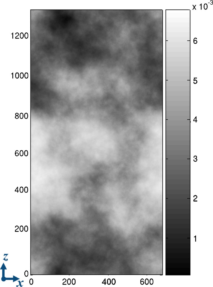
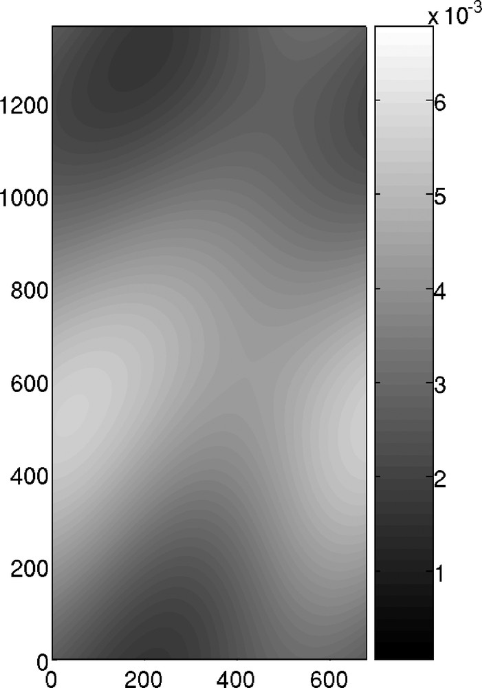
Aperture field with mean aperture A = 3.60 mm and variability of the aperture σ = 1.23 mm (σ/A = 0.34). The color bar represents the aperture in meters, the side units are plane spatial coordinates (x,z), also in meters.
Champ d’ouverture de moyenne A = 3.60 mm et de RMS σ = 1.23 mm (σ/A = 0.34). La barre de couleur indique les valeurs d’ouverture en mètres et les valeurs sur les bords sont les coordonnées spatiales (x,z), aussi en mètres.

With little knowledge about the pressure conditions along the boundaries of this model, we assume that the two facing sides along x of this rectangular fracture correspond to the inlet and outlet of the model where the pressure is homogeneous, respectively P₀ and P_lx. In other words, we assume the streamlines to be as straight as possible between both wells.

The pressure gradient ΔP/l_x is chosen as −10⁻² bar/m, which corresponds to about six bars between the bottom of both wells. The dynamic viscosity is chosen to be 3 × 10⁻⁴ Pa/s (reference value for pure water at 10 Pa and 100 °C in Spurk and Aksel (2008)). The Reynolds number rescaled with the characteristic dimensions of the fracture (Méheust and Schmittbuhl, 2001) is equal to Re′ = (ρu_x a²)/(η.l_x) = 0.026 and the Péclet number is Pe = 3.8 × 10⁴.

Then, we solve the hydraulic flow in the fracture domain and obtain the 2D velocity field, $\vec{u}$ defined in Eq. (6). Fig. 5 shows the spatial fluctuations of $| | \vec{u} | |$ . For information, a parallel plate model separated by the chosen aperture A would predict a homogeneous fluid velocity of 3.6 m/s and a thermal length R_// = 33.3 m. As we see in Fig. 5, the 2D velocity field exhibits interesting features: the fluid is rather immobile along the upper and lower borders of the fracture (close to z = 0 and z = l_x) while most of the fluid flows very quickly through a channel in the middle of the fracture.

Fig. 5
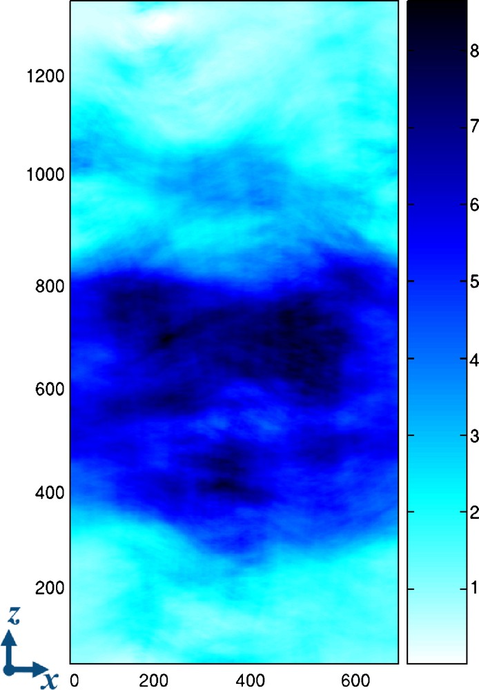
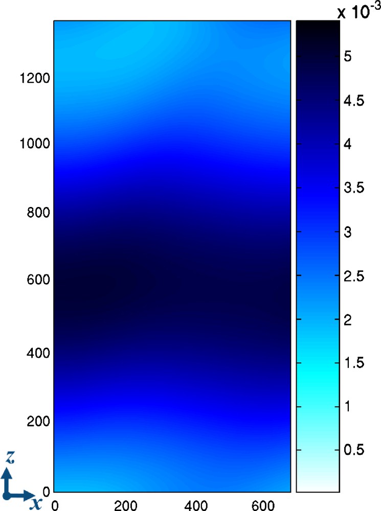
Color map of u, the 2D velocity field norm in m/s. Dark areas correspond to very high velocity while light areas show static fluid. A linear pressure gradient is imposed between the left and right of the fracture. The spatial coordinates are in meters.
Carte de u, la norme du champ de vitesse 2D en m/s. Les zones sombres correspondent à une forte vitesse tandis que les zones claires indiquent un fluide immobile. Un gradient de pression linéaire est imposé entre les bords gauche et droit de la fracture. Les coordonnées spatiales sont en mètres.

The macroscopic hydraulic aperture is deduced from the local hydraulic flow estimate (Eq. (15)): H = 3.73 mm, which is slightly higher than the mean mechanical aperture A = 3.60 mm. Therefore, this fracture is more permeable than parallel plates separated by A. In other words, the fracture is geometrically thinner than what one would expect from the knowledge of H possibly inverted from an hydraulic test. However, the local hydraulic apertures h (Eq. (16)) range from nearly 0 to 5.43 mm (Fig. 6).

Fig. 6
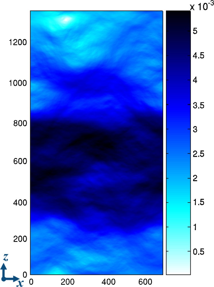
Color map of the local hydraulic aperture in metres computed from the variable aperture and velocity field shown in Figs. 4 and 5. The spatial coordinates are in meters.
Carte de l’ouverture hydraulique locale en mètres, calculée d’après le champ d’ouverture variable de la Fig. 4 et le champ de vitesse de la Fig. 5. Les coordonnées spatiales sont en mètres.

From the average estimate of the fluid velocity, we can go back to our approximation of a linear inlet, even if the fracture is not vertical and does not intersect the well on a very long distance. We might estimate this distance from the following argument. The flow rate observed at Soultz is about Q = 20 L/s. Thus, using a velocity of about u = 3.6 m/s and a fracture aperture equal to 3.6 mm implies that the well crosses such fractures over a cumulated length of about (neglecting the well radius):

L = \frac{Q}{u A} = \frac{20 \times 10^{- 3}}{3.6 \times 3.6 \times 10^{- 3}} \approx 1.5 m

which is effectively much smaller than the boundary size. However, we expect the presence of connecting fractures between the well and the fault zone to be sufficiently permeable to define an effective linear inlet of constant effective pressure. All the results presented here are valid under any dimensioning which keeps the ratio l_x/R_// constant (here equal to 20.5): for instance, the results apply for l_x = 690 m, A = 10 mm and ΔP/l_x = −1.7 × 10⁻⁴ bar/m (using the same fluid parameters), which leads to a Poiseuille velocity of about 0.46 m/s.

As we see, $\bar{T}$ is very inhomogeneous and also exhibits channeling. The chosen inlet temperature is T₀ = 60 °C, the rock temperature is T_r = 200 °C (Fig. 7) and the fluid diffusivity is χ = 0.17 mm²/s (corresponding to water at T = 100 °C, from Taine et Petit (2003). Note that the rock temperature will evolve over time in contrast to the one of our approximations. Indeed, the rock thermal diffusivity is about 1 mm²/s which is larger than the fluid diffusivity (χ = 0.17 mm²/s) but not sufficiently to be fully neglected.

Fig. 7
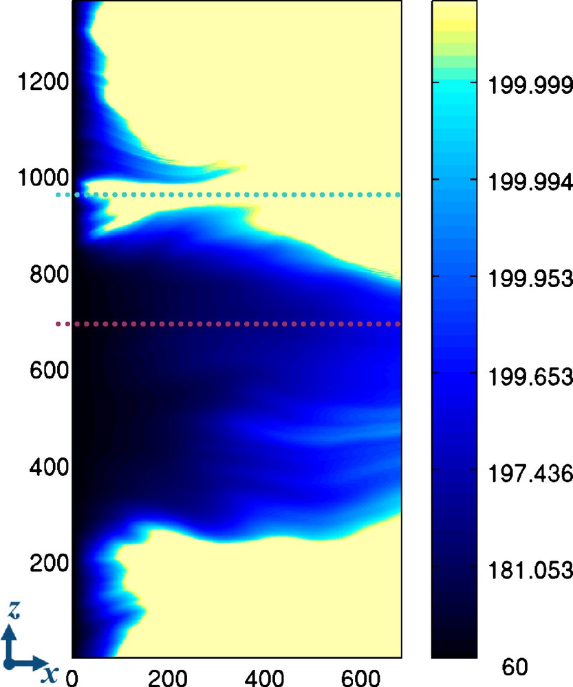
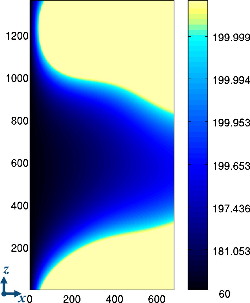
Map of the averaged temperature field $\bar{T}$ in Celsius degrees (°C). The color bar changes exponentially; thus small variations slightly below the temperature rock (200 °C) are highly visible. The dotted lines indicate the location of the profiles of temperature $\bar{T} (x, z = z_{0})$ shown in Fig. 8, for z = 960 m and z = 700 m. The spatial coordinates are in meters.
Carte du champ de température moyennée $\bar{T}$ en degrés Celcius (°C). L’échelle de couleur varie exponentiellement ; les petites variations en dessous de la température de la roche (200 °C) sont donc très visibles. Les lignes en pointillées indiquent la position des profils de température $\bar{T} (x, z = z_{0})$ montrés sur la Fig. 8, en z = 960 m et z = 700 m. Les coordonnées spatiales sont en mètres.

However, $\bar{T}$ is rather different from a parallel plate solution. Indeed, the solution is not invariant in $\hat{z}$ . Different temperature profiles function of x are shown in Fig. 8. Two end-member types of behavior are plotted: temperature profiles at z = 960 m (curve iv) and z = 700 m (curve v). The temperature difference can be larger than 100 °C in the inlet region. Even rather far from the inlet, for example at x = 200 m, the temperature difference can still be of the order of 17 °C (200.0 °C for z = 960 m, and 183.4 °C for z = 700 m). The temperature field T(x,y,z = 700 m) for this set of parameters is shown in Fig. 3, where we see how the temperature evolves along the x-axis, away from the mean plane. Temperature profiles can be compared to the one obtained for a parallel plate model where plates are separated by the aperture A (curve iii) which reads from Eqs. (13) and (17): ${\bar{\bar{T}}}_{/ /} = {\bar{T}}_{/ /}$ .

Fig. 8
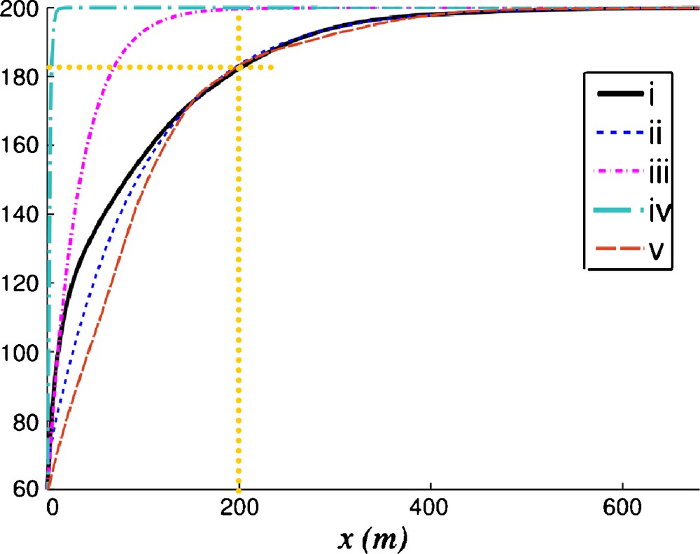
Fluid 1D temperature in °C as function of x. The continuous curve (i) shows the computed temperature $\bar{\bar{T}}$ . The dashed curve (ii) is the fit of curve (i) with an exponential function. The dot dashed curve (iii) is the fluid 1D temperature by neglecting the self-affinity perturbation (inside flat parallel plates). The curves (iv) and (v) are the profiles of temperature $\bar{T} (x, z = z)$ for respectively z = 960 m and z = 700 m (Fig. 7).
Température 1D en degrés en fonction de x. La courbe continue (i) est le profil calculé $\bar{\bar{T}}$ . La courbe tiretée (ii) est la régression de la courbe (i) avec une fonction exponentielle. La courbe (iii) est la température 1D obtenue en négligeant la perturbation auto-affine (modèle de plaques parallèles). Les courbes (iv) et (v) sont les profils de température $\bar{T} (x, z = z)$ respectivement en z = 960 m et z = 700 m (Fig. 7).

Following this model (curve iii), the fluid should be at 199.7 ̊C at x = 200 m. If we compare ${\bar{\bar{T}}}_{/ /}$ to the averaged observed temperature $\bar{\bar{T}}$ (defined in Eq. (13)) (Fig. 8, curve i), we see that ${\bar{\bar{T}}}_{/ /}$ is not representative of the end-member types of behavior. We model $\bar{\bar{T}}$ by using an adapted parallel law ${\bar{\bar{T}}}_{\mod}$ (curve ii), which is an exponential law with a suitable thermal length R:

{\bar{\bar{T}}}_{\mod} = (T_{0} - T_{r}) \exp (- \frac{x - x_{0}}{R}) + T_{r}

(19)

where R = 97 m (i.e. 2.9 × R_//) and x₀ = −10 m. As we do a least square fit on a semi-log space to obtain the parameters R and x₀, the beginning of the fit in the linear-linear space is not accurate. We see that the distance between wells (600 m in our case study) is about six times larger than R. However, owing to channeling the fluid temperature will not necessarily be in full equilibrium with the rock temperature at the out well. The thermal aperture is equal to Γ = 4.7 mm, which is rather different from the geometrical aperture A = 3.6 mm. A larger thermal aperture (compared to the geometrical one) means an inhibited thermalization on average.

3.2 Temperature estimation with few parameters

The knowledge of the spatial correlations rather than all the details of the geometrical aperture seems to be a key parameter to evaluate the hydraulic flow and the temperature of the fluid in a rough fracture. Indeed, the macroscopic geometrical aperture A brings too little information to characterize the heat exchange at the fracture scale. By contrast, it is impossible in particular for field measurements to know in detail the spatial variability of the local geometrical aperture A. Therefore, we propose to characterize the macroscopic geometrical properties with more than a single value, using several parameters describing the largest spatial variations. Numerically, it is possible to obtain them by filtering the fracture aperture field in the Fourier domain.

Fig. 9 shows the aperture field displayed in Fig. 4 once it has been filtered with the following criterion: only the Fourier coefficients fulfilling

{(\frac{k_{x}}{2 π} l_{x})}^{2} + {(\frac{k_{z}}{2 π} l_{z})}^{2} < 2^{2}

(20)

are kept, where k_x and k_z are the wave vector coordinates along respectively the x and z-axes. Since the Fourier transform is discrete, it means that we only keep the Fourier components corresponding to the wave number

(n_{x}, n_{z}) = (2 π / (k_{x} . l_{x}), 2 π / (k_{z} . l_{z}))

in {(0,0);(0,1);(1,0);(1,1)} (i.e. the average A and the first Fourier modes along x and z are left).

Fig. 9
Map of the coarse-grained fracture aperture in metres, obtained by a very low pass filtering of the aperture (Fig. 4) keeping only the zero and first Fourier modes along x and z. The spatial coordinates are in meters.
Carte de l’ouverture géométrique à faible résolution spatiale, en mètres, obtenue en filtrant l’ouverture (Fig. 4), en ne gardant que la moyenne et les premiers modes de Fourier sur x et z. Les coordonnées spatiales sont en mètres.

Let us assume that we only have these data available to evaluate the hydraulic flow and heat exchange. Using the same method and the same parameters as previously, we compute the pressure field corresponding to the filtered aperture field. In Fig. 10, we show the hydraulic aperture field we obtain. As we see, the high hydraulic aperture channel in the middle of the figure remains, while high frequency variations are removed. These large scale fluctuations of the hydraulic flow, computed from the knowledge of a very limited set of Fourier modes of the geometrical aperture, might be obtained from field measurements. Then, the corresponding temperature field shown in Fig. 11 is computed. The main features of the thermal field (Fig. 7) are still visible: the main channel is at the same position and the values are of the same order of magnitude. Despite small local differences, this substitution model gives a relevant description of what thermally happens.

Fig. 10
Map of the local hydraulic aperture in meters, obtained from the filtered geometrical aperture shown in Fig. 9. This figure has to be compared to Fig. 6 (same color bar). The spatial coordinates are in meters.
Carte de l’ouverture hydraulique en mètres obtenue d’après les ouvertures géométriques filtrées de la Fig. 9. Ce champ est comparable à celui de la Fig. 6 (même échelle de couleur). Les coordonnées spatiales sont en mètres.

Fig. 11
Map of the temperature field obtained using the previous coarse-grained aperture and its corresponding hydraulic results (Figs. 9 and 10). The color scale is in °C and it changes exponentially. The spatial coordinates are in meters.
Carte de température obtenue en utilisant les ouvertures filtrées et les résultats hydrauliques correspondant (Fig. 9 et 10). L’échelle de couleur, en °C, varie exponentiellement. Les coordonnées spatiales sont en mètres.

4 Conclusions

We propose a numerical model to estimate the impact of the fracture roughness on the heat exchange at the fracture scale between a cold fluid and the hot surrounding rock. We assume the flow regime to be permanent and laminar. The numerical model is based on a lubrication approximation for the fluid flow (Reynolds equation). We also introduce a “thermal lubrication” approximation, which leads to a quartic profile of the temperature across the aperture. It is obtained by assuming that the in-plane convection is dominant with respect to the in-plane conduction (i.e. high in-plane Péclet number). The lubrication approximation implies also that the off-plane convection is neglected; subsequently, the heat conduction initiated by the temperature difference between the rock and the fluid is supposed to be the major off-plane phenomenon.

Our model shows that the roughness of the fracture can be responsible for fluid channeling inside the fracture. In this zone of high convection, the heat exchange is inhibited, i.e., the fluid needs a longer transport distance to reach the rock temperature. Spatial variability of the temperature is characterized on average by a thermal length and a thermal aperture.

In this article, we illustrate our modeling by a case study at the geothermal reservoir of Soultz-sous-Forêts, France, with a rough aperture which leads to inhibited thermal exchanges owing to a strong channeling effect, in the sense that the characteristic thermal length in this stationary situation is longer in rough fractures than in flat ones with the same transmissivity. Qualitatively, this can be attributed to the localization of the flow inside a rough fracture: most of the fluid flows through large aperture zones at faster velocity than the average, which leads to longer thermalization distances.

We performed simulations for about 1000 other aperture fields (not illustrated here) compatible with the macroscopic observations, of the same type as shown here. A general property holds for all these aperture fields: the thermal exchanges are always inhibited in rough fractures, compared to a fracture modeled by parallel plates with the same macroscopic hydraulic transmissivity (Neuville et al., submitted) (same H).

From the numerical solutions, we see that the mean geometrical aperture provides too little information to characterize the variability of the fluid flow and fluid temperature. In contrast, the knowledge of the dominant spatial variation of the geometrical aperture field (here obtained by keeping only the largest scale fluctuations using low pass Fourier filtering) provides interesting information about the spatial pattern of the hydraulic and thermal fields. The macroscopic spatial correlation of the aperture is shown to be an important parameter ruling the hydrothermal behavior. Note that we considered a self-affine model for the aperture roughness, but other types of geometrical descriptions of this roughness (given either by constraints from field measurements, or other kind of geometrical models), could be also considered using the type of simulations described here.

Acknowledgements

We thank Albert Genter, Reinhard Jung Marion, Patrick Nami, Marion Schindler, Eirik G. Flekkøy, Stéphane Roux, Jose S. Andrade Jr. and Yves Méheust for fruitful discussions. This work has been supported by the EHDRA project, the REALISE program and the French Norwegian PICS project.

¹ We compared our method to another algorithm based on a Lattice Boltzmann (LB) method, which does not reduce Navier-Stokes to a Stokes equation and does not hypothesize any lubrication approximation, in order to solve the velocity and temperature fields. The finite diffusivity of the rock is also taken into account. From those results, it appears that the analytical parabolic and quartic approximations (with the proper coefficients) of the respective fields are indeed consistent within a 5% error bar with the LB results.

Bibliographie

[Al-Yaarubi et al., 2005] Al-Yaarubi, A.H., Pain, C.C., Grattoni, C.A., Zimmerman, R.W., 2005. Navier-Stokes simulations of fluid flow through a rock fracture, Dynamics of fluids and transport in fractured rock, AGU Monograph 162 ed. by B. Faybishenko, P.A. Witherspoon, and J. Gale, Amer. Geophys. Union, Washington, DC, pp. 55–64.

[Bachler et al., 2003] D. Bachler; T. Kohl; L. Rybach Impact of graben parallel faults on hydrothermal convection – Rhine graben case study, Phys. Chem. Earth, Volume 28 (2003), pp. 431-441

[Bataillé et al., 2006] A. Bataillé; P. Genthon; M. Rabinowicz; B. Fritz Modeling the coupling between free and forced convection in a vertical permeable slot: Implications for the heat production of an Enhanced Geothermal System, Geothermics, Volume 35 (2006), pp. 654-682

[Batchelor, 2002] G.K. Batchelor An introduction to fluid dynamics, Cambridge University Press, Cambridge, UK, 2002 (615 p)

[Boffa et al., 1998] J.M. Boffa; C. Allain; J.P. Hulin Experimental analysis of fracture rugosity in granular and compact rocks, Eur. Phys. J. Appl. Phys., Volume 2 (1998), pp. 281-289

[Bouchaud, 1997] E. Bouchaud Scaling properties of cracks, J. Phys. Cond. Matter, Volume 9 (1997), pp. 4319-4344

[Brown, 1987] S.R. Brown Fluid flow through rock joints: the effect of surface roughness, J. Geophys. Res., Volume 92 (1987), pp. 1337-1347

[Brown and Scholz, 1985] S.R. Brown; C.H. Scholz Broad bandwidth study of the topography of natural rock surfaces, J. Geophys. Res., Volume 90 (1985), pp. 12575-12582

[Cox and Wang, 1993] B.L. Cox; J.S.Y. Wang Fractal surfaces: measurement and application in earth sciences, Fractal, Volume 1 (1993), pp. 87-115

[Ge, 1998] S. Ge Estimation of groundwater velocity in localized fracture zones from well temperature profiles, J. Volcanol. Geothermal Res., Volume 84 (1998), pp. 93-101

[Gentier, 2005] Gentier, S., Rachez, X., Dezayes, C., Hosni, A., Blaisonneau, A., Genter, A. Bruel, D., 2005. Thermohydro-mechanical modelling of the deep geothermal wells at Soultz-sous-Forêts, Proceedings of EHDRA scientific conference.

[Gérard et al., 2006] A. Gérard; A. Genter; T. Kohl; P. Lutz; P. Rose; F. Rummel The deep EGS (Enhanced geothermal System) project at Soultz-sous-Forêts (Alsace, France), Geothermics, Volume 35 (2006), pp. 473-483

[Heuer et al., 1991] N. Heuer; T. Küpper; D. Windelberg Mathematical model of a Hot Dry Rock system, Geophys. J. Int., Volume 105 (1991), pp. 659-664

[Iwai, 1976] Iwai, K., 1976. Fundamental Studies of Fluid Flow through a single fracture, Ph.D. Thesis, University of California, Berkeley.

[Kolditz and Clauser, 1998] O. Kolditz; C. Clauser Numerical simulation of flow and heat transfer in fractured cristalline rocks: application to the hot dry rock site in Rosemanowes (U.K.), Geothermics, Volume 27 (1998), pp. 1-23

[Landau and Lifchitz, 1994] L. Landau; E. Lifchitz Physique théorique mécanique des fluides, Ed. MIR-Ellipses, Paris, France, 1994 (280 p)

[Méheust, 2002] Méheust, Y., 2002. Écoulements dans les fractures ouvertes, Ph.D. thesis Université Paris Sud.

[Méheust and Schmittbuhl, 2000] Y. Méheust; J. Schmittbuhl Flow enhancement of a rough fracture, Geophys. Res. Lett., Volume 27 (2000), pp. 2989-2992

[Méheust and Schmittbuhl, 2001] Y. Méheust; J. Schmittbuhl Geometrical heterogeneities and permeability anisotropy of rough fractures, J. Geophys. Res., Volume 106 (2001), pp. 2089-2102

[Méheust and Schmittbuhl, 2003] Méheust, Y., Schmittbuhl, J., 2003. Scale effects related to flow in rough fractures, PAGEOPH 160, 1023–1050.

[Neuman, 2005] S. Neuman Trends, prospects and challenges in quantifying flow and transport through fractured rocks, Hydrogeol. J., Volume 13 (2005), pp. 124-147

[Neuville et al., submitted] Neuville, A., Toussaint, R., Schmittbuhl, J., Hydrothermal coupling in a self-affine rough fracture, submitted to PRE (2010).

[Pinkus and Sternlicht, 1961] O. Pinkus; B. Sternlicht Theory of hydrodynamic Lubrication, Mc Graw-Hill, New York, 1961 (465 p)

[Plouraboué et al., 2000] F. Plouraboué; P. Kurowski; J.M. Boffa; J.P. Hulin; S. Roux Experimental study of the transport properties of rough self-affine fractures, J. Contaminant Hydrology, Volume 46 (2000), pp. 295-318

[Power et al., 1987] W.L. Power; T.E. Tullis; S.R. Brown; G.N. Boitnott; C.H. Scholz Rhougness of natural fault surfaces, Geophys. Res. Lett., Volume 14 (1987), pp. 29-32

[Press et al., 1992] W.H. Press; S.A. Teukolsky; W.T. Vetterling; B.P. Flannery Numerical Recipes, Cambridge University Press, New York, USA, 1992 (994 p)

[Rachez et al., 2007] Rachez, X., Gentier, S., Blaisonneau, A., 2007. Current status of BRGM modeling activities at the Soultz EGS reservoir: hydro-mechanical modeling of the hydraulic stimulation tests and flow and transport modelling of the in-situ tracer test, proceedings of EHDRA scientific conference.

[Roux et al., 1993] S. Roux; J. Schmittbuhl; J.P. Vilotte; A. Hansen Some physical properties of self-affine rough surfaces, Europhys. Lett., Volume 23 (1993), pp. 277-282

[Sanjuan et al., 2006] B. Sanjuan; J.L. Pinault; P. Rose; A. Gerard; M. Brach; G. Braibant et al. Tracer testing of the geothermal heat exchanger at Soultz-sous-Forets (France) between 2000 and 2005, Geothermics, Volume 35 (2006), pp. 622-653

[Santucci et al., 2007] Santucci, S., Måløy, K.J., Delaplace, A., Mathiesen, J., Hansen, A. Haavig Bakke, J.Ø., Schmittbuhl, J., Vanel, L., Ray, P., 2007. Statistics of fracture surfaces, Physical Review E 75, 016104 6p.

[Sausse et al., 2008] Sausse, J., Dezayes, C., Genter, A., Bisset, A., 2008. Characterization of fracture connectivity and fluid flow pathways derived from geological interpretation and 3D modelling of the deep seated EGS reservoir of Soultz (France), Proceedings, thirty-third workshop on Geothermal Reservoir Engineering, Stanford, California.

[Schmittbuhl et al., 1993] J. Schmittbuhl; S. Gentier; S. Roux Field measurements of the roughness of fault surfaces, Geophys. Res. Lett., Volume 20 (1993), pp. 639-641

[Schmittbuhl et al., 1995] J. Schmittbuhl; F. Schmitt; C. Scholz Scaling invariance of crack surfaces, J. Geophys. Res., Volume 100 (1995), pp. 5953-5973

[Schmittbuhl et al., 2008] J. Schmittbuhl; A. Steyer; L. Jouniaux; R. Toussaint Fracture morphology and viscous transport, Int. J. Rock Mech. Min. Sci., Volume 45 (2008), pp. 422-430

[Spurk and Aksel, 2008] J.H. Spurk; N. Aksel Fluid Mechanics, Springer, Berlin, Germany, 2008 (516 p)

[Stokes, 1846] G.G. Stokes On the theories of the internal friction of fluids in motion, and of the equilibrium and motion of elastic solids, Trans. Cambr. Phil. Soc, Volume 8 (1846), pp. 287-319

[Taine and Petit, 2003] J. Taine; J.P. Petit Transferts thermiques, Dunod, Paris, France, 2003 (449 p)

[Tsang and Tsang, 1998] Y.W. Tsang; C.F. Tsang Flow channeling in a single fracture as a two-dimensional strongly heterogeneous permeable medium, Water Resour. Res., Volume 25 (1998), pp. 2076-2080

[Turcotte and Schubert, 2002] D.L. Turcotte; G. Schubert Geodynamics, Cambridge University Press, Cambridge, UK, 2002 (pp. 262–264)

[Zimmerman et al., 1991] R.W. Zimmerman; S. Kumar; G.S. Bodvarsson Lubrication Theory Analysis of Rough-Walled Fractures, Int. J. Rock. Mech., Volume 28 (1991), pp. 325-331

Commentaires - Politique

Ces articles pourraient vous intéresser

Miscible transfer of solute in different model fractures: From random to multiscale wall roughness

Harold Auradou; Alejandro Boschan; Ricardo Chertcoff; ...

C. R. Géos (2010)

3D model of fracture zones at Soultz-sous-Forêts based on geological data, image logs, induced microseismicity and vertical seismic profiles

Judith Sausse; Chrystel Dezayes; Louis Dorbath; ...

C. R. Géos (2010)