

1 Introduction
Most of the water supply in Denmark is provided by groundwater; therefore, the Danish Government is interested in maintaining groundwater quality to avoid complex and expensive treatment processes. As contamination from domestic, industrial and agricultural activities threatens the groundwater resources, several ambitious plans have been adopted by the Danish Government in order to protect the high quality groundwater and to meet future water supply challenges [2,19]. In accordance with these plans, detailed hydrogeological mapping has been demanded by the Danish Environmental Protection Agency (EPA).
Until recently, primary information available for the geology and groundwater in Denmark was borehole data. However, even in areas with a high density of boreholes, existing hydrogeological mapping based exclusively on borehole data turned out to be inadequate. Consequently, dense geophysical mapping of the subsurface has become a central discipline in hydrogeological mapping. Geophysical mapping is performed primarily with the aim of determining the extent of the aquifers and their vulnerability.
Pulled Array Continuous Electrical Sounding (PACES), Continuous Vertical Electrical Sounding (CVES), borehole logging, Seismic and especially Time Domain ElectroMagnetics (TDEM), ground and airborne, i.e. SkyTEM geophysical methods are frequently used in Denmark. Moreover, geophysical results are often used in groundwater modelling when borehole data are not available.
The Magnetic Resonance Sounding (MRS) method differs from traditional surface-based geophysical methods by measuring a signal generated directly by groundwater molecules. Thus, it could be extremely relevant as an additional geophysical tool in Denmark.
2 MRS campaigns in Denmark
In 2003, the first MRS test campaign was carried out in the northern part of Denmark, with the aim of testing the applicability of the method. The survey was planned by Hydrogeophysics Group of Århus University (HGG) and Institute for Research and Development, France (IRD). A high level of artificial electromagnetic noise was observed during the survey, due to the country-specific constraints. A second MRS test campaign was conducted in May 2006 by the Danish company Rambøll in cooperation with the former County of Vejle (Denmark), Paris 6 University and IRD (both France). The MRS results obtained suggest optimal locations for water supply boreholes within subsurface structures with homogeneous electrical resistivity conditions mapped by TDEM [2]. An optimisation procedure during field measurements made it possible to obtain good quality MRS data and the method was thereby optimised to fit the Danish conditions.
Based on these results, a third campaign was planned and conducted by Rambøll in cooperation with the Environmental Centre Århus, Odense and Ringkøbing in November 2007 in different geological settings.
In total, between 2003 and 2007, 12 sites were investigated with MRS in Denmark (Fig. 1). At two sites (Kragelund and Sæby), it was impossible to measure with MRS due to the high level of ambient electromagnetic noise. A total of 47 MRS stations were measured in Denmark between 2003 and 2007. During all three campaigns, NUMISPLUS equipment from IRIS Instruments was used. Measurement procedures and configurations were adapted according to each site's specific constraints (ambient noise, required depth resolution) [2].

Location of MRS sites in Denmark from 2003 to 2007.
Localisation des sites RMP au Danemark du 2003 au 2007.
3 Geology and hydrogeology of the investigated areas
The Danish landscape was formed by glacial activity during the Weichselian ice age and the geology is composed mainly of glacial sedimentary structures. The south-western part of Jutland is dominated by glacial melt water plains with sandy sediments and sandy soil from old moraine landscapes of the Saale glaciation. The rest of Jutland and the Danish isles are generally built up of moraine landscape with sediments deposited through melting of the Weichselian ice [17,18]. The Quaternary sediments consist of moraine-clay, -sand and -gravel as well as fluvio-glacial-clay, -sand and -gravel. These Quaternary sediments overlie mica sediments, sand, clay and limestone from the Tertiary and Cretaceous.
Aquifers in Denmark are mainly found in glacial Quaternary melt water sediments, deep Tertiary sandy formations and in Cretaceous and Palaeocene limestone. Aquifers in the deep Tertiary sandy formations are often regional aquifers, but aquifers in limestone and glacial sediments can be both regional and local. The glacial aquifers in the eastern part of Jutland are often found in buried valleys eroded into the Tertiary clays and can be rather complex with a primary and several secondary aquifers, consolidated and unconsolidated.
A short description of the aquifers within the investigated areas, according to the geology and the hydrogeology of the areas [6] and available description of boreholes [5], is presented in Table 1.
Brève description des aquifères à partir des données de forages disponibles pour chaque site étudié.
| Location | Site | Short description of aquifers from available borehole data |
| Northern Jutland | Høgsted | Mainly one aquifer in fine melt water sand |
| Næsby | Aquifers in fine sand. Deeper aquifers in limestone | |
| Sæby | Mainly one aquifer in fine melt water sand in buried valley structure | |
| Lemvig | Three aquifers. The top is medium sand with coarse grains and unconfined. The second aquifer is in fine to medium sand and confined. Between the two top aquifers are silt and clay. The primary deepest aquifer is below 100 m depth in medium sand | |
| Central and southern Jutland | Bredal | One confined aquifer in medium and coarse sand, and in some cases in mica sand |
| Lindved | One main confined aquifer in a thin layer of gravel or thick layer of mica sand. Secondary aquifers exist | |
| Kragelund | One confined aquifer in fine to medium sand and gravel. Secondary aquifers exist | |
| Dalby | One confined aquifer in medium to coarse sand. Small secondary aquifers exist | |
| Lyngby | One confined aquifer in medium sand to gravel. Secondary aquifers exist | |
| Funen | Søndersø | Regional main confined to semi-confined aquifer in melt water sediments inside a buried valley. Fine and medium sand to gravel. A confined to semi-confined secondary aquifer is present in the whole area |
| Small islands | Ærø | Three thin aquifers that are not all present everywhere. Fine to medium clayey sand |
| Samsø | No regional aquifers, only local aquifers in medium sand and moraine clay |
4 MRS method and parameters obtained
The MRS method is based on the property of the nuclei of the hydrogen atoms (protons) in groundwater molecules to possess a magnetic moment. These moments are excited using a surface loop with current passing through. The magnetic resonance signal generated by the precessing nuclei is measured, with the same loop, after the current cut-off. The amplitude of the signal is proportional to the number of hydrogen nuclei of water molecules that generate the signal, and the decay of the signal is linked to the mean size of the pores that contain the water. The basics of the method are discussed in [11].
The geophysical parameters derived from the magnetic resonance signal are the MRS water content () and the relaxation times ( and T1) versus depth. is defined as the volume of water with a sufficiently long decay time constant (>30 ms) per unit volume [12]. Signals with short decay time constants are generated by bound-water, i.e. water that is attached to the rocks due to the forces of molecular attraction, which cannot be measured.
Both T1 and are linked to the mean pore size containing water but is influenced by the local heterogeneities of the local magnetic field [11]. Thus, T1 is a more reliable parameter, usually called the longitudinal relaxation time, which is linked to the mean pore size of the aquifer as [7,8]:
| (1) |
and T1 are used to estimate the hydraulic conductivity () and the transmissivity () of aquifers [13,15] as follows:
| (2) |
| (3) |
Different schemes are known for MRS data inversion [1,3,4,16]. However, the resolution of the inversion is not defined by the inversion algorithm but by the physical basis of the method and the signal to noise ratio. For MRS data inversion in this study, the SAMOVAR software based on the Tikhonov regularization method [10] was used. This software allows processing of complex signals (amplitude and phase). It is possible to use either the “smooth” inversion or the “block” inversion schemes. The software allows automatic estimation of the uncertainty in MRS results based on the eigenvalues of the matrix that approximates the MRS integral equation [14].
An example is presented in Fig. 2, where automatic “smooth” and “block” inversion were used for Bredal-4 MRS station data inversion. Both schemes fit raw data equally well (0.6% fitting error for smooth inversion and 1.5% fitting error for block inversion).
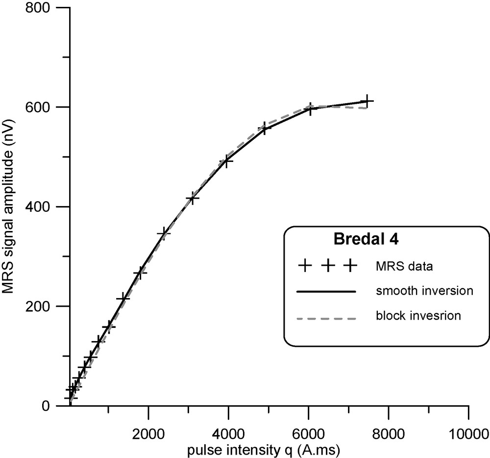
Fitting Bredal-4 MRS data using automatic “block” and “smooth” inversion.
Lissage de données RMP pour la station Bredal-4 avec « block » et « smooth » inversions automatiques.
Inversion results (, T1 and ) using “smooth” and “block” inversion schemes for Bredal-4 MRS station are presented in Fig. 3. For estimation, the calibration constant, , previously calculated for this site [2], is used. The MRS depth resolution uncertainty is also shown. This graph makes it possible to estimate the uncertainty of aquifer resolution within with respect to the Signal / Noise ratio [14]. Both inversion scheme results are acceptable.
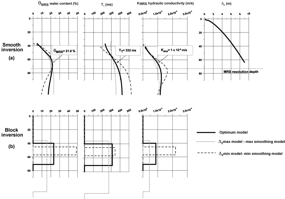
MRS water content , decay time T1 and hydraulic conductivity obtained after (a) “smooth” inversion and (b) “block” inversion for the Bredal-4 MRS stations. For calculation [1] is used.
Teneur en eau , temps de décroissance T1 et conductivité hydraulique obtenus, avec (a) inversion « smooth » et (b) inversion « block » pour Bredal-4 station RMP. Pour le calcul , la valeur [1] est utilisée.
The regularization method provides the unique solution that is selected based on the signal-to-noise estimation. As noise is not necessarily constant, selection of the minimum and maximum values of the parameter of regularization provides a solution between the maximum and the minimum water content (Fig. 3a). For each depth (), the water content derived from the inverse model can be attributed to the depth ().
When using the “block” inversion scheme, we stabilise the solution by defining the minimum number of blocks. For this example (Fig. 3b), we selected a one-block solution that allows fitting raw data within the noise magnitude. However, even selecting one block we obtain the minimum and maximum thickness solutions both of which fit the experimental data within the noise magnitude (Fig. 3b). Thus, for the “block” inversion, the uncertainty is given directly. Comparison of the inversion results obtained by “smooth” and “block” inversion presented in Fig. 3 shows that the “smooth” inversion is closer to the maximum thickness solution given by the “block” inversion. Even if the “block” inversion scheme provides a rectangle with well-defined thickness and water content, “block” inversion is not more accurate than “smooth” inversion because of the many other different rectangles which can fit experimental data equally well. As we have no other information about the solution (e.g. number of water-saturated layers, static water level, bottom of the aquifer), except the signal-to-noise ratio, we use the “smooth” inversion scheme.
In the present study, the “smooth” inversion of complex signal routine was used. For “smooth” inversion, T1 corresponds to the maximum value of the inversion curve (Fig. 3a).
5 Simplified classification of aquifer grain-size
Within the investigated sites, aquifers can be found mainly in melt water sandy sediments and on a few rare occasions in clayey melt water and moraine sediments [5,6]. In order to compare the MRS parameters obtained with the available geological data, a qualitative classification of the aquifer grain-size was attempted, based on the geological description of boreholes (corresponding depth of the installed screen).
From the borehole descriptions [5], four main classes of aquifers can be recognised within the investigated sites: moraine clay (MCl), fine sand (FS), medium sand (MS) and coarse sand (CS). Three intermediate classes within the main classes are also considered (MCL-FS, FS-MS, MS-CS). This grain-size classification based entirely on the available borehole data is qualitative due to the absence of detailed grain-size analyses. Hence, to improve the legitimacy of the aquifer classification, an arbitrary uncertainty error () was estimated as follows:
| (4) |
is a factor related to the hydrogeological variability in the area of the borehole; regional aquifer: , local aquifer: .
is the uncertainty related to the geological description of the borehole: good description: , fair description: , poor description: the borehole is not used for comparison.
is a factor related to the year of the drilling before and after the Danish guide for borehole sample description [9] published in 1995. After 1995: ; before 1995: .
An upper limit of 500 m distance for comparison was chosen based on an assessment of average hydrogeological variability [6] of the specific investigated sites. Increased age of the borehole and only fair borehole description increases the uncertainty of the aquifer class, since the description of the grain-size in these cases is considered less accurate. The attributed percentage of uncertainty may be inexact because the formula is empirical and values are based on several hydrogeological assessments and evaluations.
We demonstrate this approach by using the example of MRS station Bredal-4 and DGU-borehole 116.1624 (Fig. 4). Bredal-4 MRS inversion results ( and ) are compared with TDEM sounding results. The MRS depth resolution uncertainty is also shown. The borehole's screen was set within sediments described as medium to coarse sand. Thus, the attributed class is MS-CS. The borehole was drilled in 2006 and the quality of the geological description is good. However, as the borehole is situated at a distance of 500 m from the MRS station and the aquifer is considered regional, the uncertainty error of 25% on the grain-size classification was prescribed.
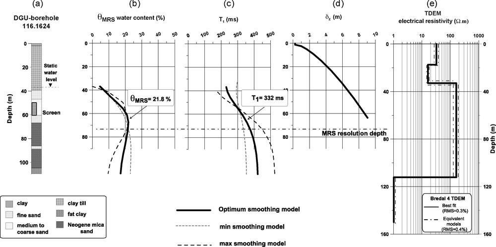
(a) 116.1624 DGU-borehole log [5]; (b) Bredal-4 MRS station results: water content , relaxation time T1 and MRS depth resolution uncertainty and (c) TDEM geoelectrical model.
(a) Description du forage DGU 116.1624 [5] ; (b) résultats RMP Bredal-4 : teneur en eau , temps de décroissance T1 et incertitude sur la profondeur de résolution et (c) modèle géoélectrique TDEM.
For our study, only 23 MRS stations have a borehole with an acceptable geological description within a distance of 500 m. Comparison is made for these MRS stations with the simplified classification of the aquifer at the depth of the screen in the adjacent DGU-borehole.
6 Comparison of results
6.1 MRS parameters
In Table 2, and T1 (optimum, maximum and minimum values) for 23 MRS stations, near DGU-boreholes, estimated classification and the are presented. The minimum and maximum values of and T1 are provided using inversion with maximum and minimum values of the regularisation parameters respectively, given by Tikhonov regularisation method based on estimation of the signal-to-noise ratio [10]. The estimated classification at the depth of the screen in the borehole is compared to the MRS values at the corresponding depth. In areas where more than one aquifer is present, a comparison is made only for the first aquifer due to the greater uncertainty in the MRS parameters for the second aquifer.
Paramètres RMP ( et T1) et classification simplifiée selon la granulométrie des aquifères, d’après les forages DGU voisins.
| MRS station | (%) | T1 (ms) | DGU boreholes number | Classification | Uncertainty (%) | ||||
| Opt. | Min. | Max. | Opt. | Min. | Max. | ||||
| ÆRO 1 | 7.6 | 6.2 | 10.4 | 208.5 | 186.6 | 227.5 | 171.112 | MCL-FS | 16 |
| ÆRO 3 | 9.6 | 7.5 | 11.2 | 227.6 | 225.8 | 238.3 | 171.21; 117.33 | FS | 56 |
| ÆRO 4 | 9.2 | 8.7 | 14 | 244.6 | 255.3 | 241.4 | 171.59 | FS | 31 |
| ÆRO 5 | 4.6 | 3.6 | 7.8 | 219 | 197.7 | 235.9 | 171.98 | FS | 31 |
| BREDAL 1 | 20.6 | 18.1 | 25 | 173.6 | 161.3 | 194.3 | 116.286; 116.917 | FS-MS | 25 |
| BREDAL 2 | 20.3 | 20.6 | 21.5 | 223.2 | 219.8 | 225.7 | 116.291; 116.1007 | MS-CS | 25 |
| BREDAL 3 | 32.5 | 32.4 | 28.7 | 320.6 | 312.5 | 348.8 | 116.811; 116.114; 116.1208 | MS-CS | 50 |
| BREDAL 4 | 21.8 | 22.9 | 20 | 332.6 | 314.3 | 342.3 | 116.1624 | MS-CS | 25 |
| DALBY 1 | 26.8 | 23.9 | 30.5 | 407.1 | 398.6 | 417.2 | 134.1477 | CS | 25 |
| DALBY 3 | 20.4 | 17.2 | 25.3 | 366.9 | 295.5 | 462.1 | 134.720 | MS-CS | 50 |
| HØGSTED 5 | 15.4 | 12 | 16.5 | 269 | 234.7 | 283 | 9.933 | FS | 25 |
| LEMVIG 1 | 26.9 | 21.5 | 30.8 | 268.2 | 265.2 | 280.6 | 53.367; 53.679 | MS | 25 |
| NÆSBY 1 | 6.1 | 4.4 | 8.3 | 146.5 | 135 | 160 | 32.640 | MCL | 50 |
| SAMSØ 1 | 19.1 | 16.3 | 24.9 | 404 | 394.2 | 440.3 | 109.72; 109.183; 109.182 | MS-CS | 31 |
| SAMSØ 4 | 15.2 | 12.3105 | 20.7 | 388 | 366.4 | 410.6 | 109.54; 109.229 | MS | 56 |
| SAMSØ 5 | 17.4 | 16.7 | 20.7 | 396.4 | 372.2 | 421.8 | 109.176; 109.27; 109.69 | CS | 56 |
| SAMSØ 6 | 13.1 | 12.3 | 13.7 | 323.5 | 317.9 | 325.2 | 109.206 | FS | 56 |
| SØNDERSØ 3 | 23.6 | 20.0 | 24.8 | 207.2 | 189.5 | 250 | 136.382 | MS-CS | 25 |
| SØNDERSØ 4 | 8.2 | 7.1 | 10.7 | 382 | 400.6 | 390 | 136.126 | FS | 25 |
| SØNDERSØ 5 | 22.8 | 21.5 | 27.4 | 410 | 379.2 | 424.6 | 136.388; 136.382 | MS-CS | 25 |
| SØNDERSØ 7 | 17.0 | 15.8 | 20 | 343.2 | 305.1 | 358.6 | 136.323; 136.335 | MS | 50 |
| SØNDERSØ 10 | 18.6 | 16.6 | 21.3 | 245.7 | 239.7 | 267.5 | 136.857 | FS-MS | 25 |
| SØNDERSØ 11 | 27.2 | 22.9 | 32.9 | 384.9 | 300.8 | 399.8 | 136.343; 136.380 | MS-CS | 25 |
and T1 for each site are plotted against the grain-size class of the aquifer (Figs. 5 and 6, respectively). The MRS values are estimated using the smooth inversion results, as shown in Figs. 3 and 4. The X-axis error bar shows the estimated uncertainty of the grain-size classification. The Y-axis error bar shows the estimated uncertainty of the MRS-obtained parameters. This uncertainty corresponds to the minimum and maximum values presented in Table 2.

MRS water content against aquifer class (MCL: moraine clay; FS: fine sand; MS: medium sand; CS: coarse sand).
Teneur en eau RMP , en fonction de la classe de l’aquifère (MCL : argiles morainiques ; FS : sable fin ; MS : sable moyen ; CS : sable grossier).

MRS decay time T1 against aquifer class (MCL: moraine clay; FS: fine sand; MS: medium sand; CS: coarse sand).
Temps de décroissance RMP T1, en fonction de la classe de l’aquifère (MCL : argiles morainiques ; FS : sable fin ; MS : sable moyen ; CS : sable grossier).
We observe a tendency toward increasing MRS water content and MRS decay time for sites with aquifers in coarser sediments. Inversely, a decrease of both MRS parameters is shown in aquifers with decreasing grain-size sediments or an increasing fraction of clay.
The dispersion of the plotted data is partly due to the limited resolution of MRS and also the lack of detailed grain-size analyses from geological borehole data. Moreover, in several cases, aquifers with the same qualitative description of the grain-size exhibit a relative large range of and values.
6.2 MRS hydraulic conductivity estimator
For MRS hydraulic conductivity estimation, calibration with pumping tests from nearby boreholes is necessary. This calibration concerns mainly the local calibration factor, which depends essentially on the reservoir's nature and structure. As reliable calibration was not available at all sites in Denmark, for comparison with aquifer classes normalised values of the MRS hydraulic conductivity estimator () were used. does not allow a quantitative estimation of the hydrogeological properties of the investigated aquifers but allows qualitative comparison of the aquifers in-between. Thus, within investigated areas may vary between 0 and 1.
In Fig. 7, for each site is plotted against the grain-size class of the aquifer, in the corresponding borehole, given in Table 2 (total of 23 MRS stations). We can observe that MRS hydraulic conductivity is higher in aquifers with coarser sediments and lower in aquifers with decreasing grain-size or increasing fraction of clay. Consequently, the general rule for implanting water supply boreholes would be to select sites with larger values. This rule can also be applied to aquifers in MS–CS (medium to coarse sand) grain-size class, despite a larger dispersion of values as compared to other classes.
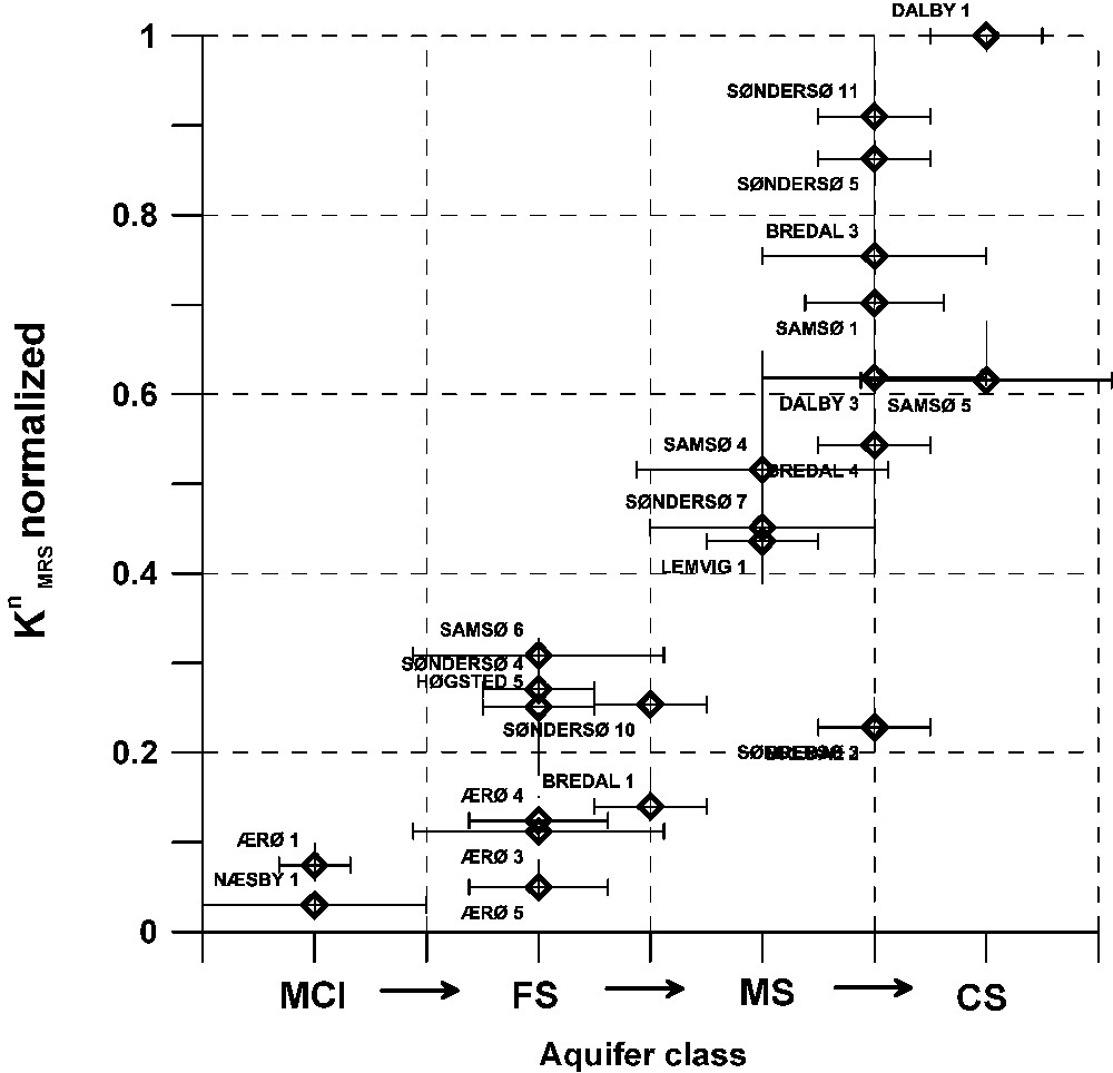
MRS hydraulic conductivity estimator against aquifer class (MCL: moraine clay; FS: fine sand; MS: medium sand; CS: coarse sand).
Estimateur de la conductivité hydraulique RMP , en fonction de la classe de l’aquifère (MCL : argiles morainiques ; FS : sable fin ; MS : sable moyen ; CS : sable grossier).
7 Discussion
To summarise the MRS results in Denmark, from 37 out of 47 MRS stations from ten successfully investigated areas are presented in Fig. 8. The excluded MRS soundings are not used due to the high uncertainty of MRS-derived parameters [2].
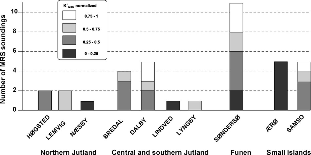
results of 37 MRS stations from 10 investigated areas.
Résultats de 37 stations RMP pour dix sites étudiés.
Using the normalised values of , we separated the aquifers into four families characterised by with an equal step of 0.25. We assumed that every family corresponds to a different range of hydraulic conductivity.
The MRS results reveal clear variations in the hydraulic conductivity within the investigated areas. In some areas, such as Søndersø, all types of different families are present. In Ærø on the other hand, mainly one family of aquifers with low hydraulic conductivity is present. Fig. 7 shows that this family corresponds mainly to clayey-fine sand aquifers.
Despite the fact that MRS transmissivity is a more robust parameter regarding equivalence problems [2], it was not used for the present study since it is also related to the aquifer thickness, . The MRS hydraulic conductivity estimator is a more appropriate parameter since it is related to the geological (grain-size) consistence of sedimentary aquifers.
8 Conclusions
Our experience shows that the MRS method is applicable in Denmark. We observed a qualitative relationship between MRS results and the grain-size class of the aquifer: larger values of MRS-derived parameters correspond to aquifers with coarser material. Thus, the MRS method seems to be able to provide a qualitative estimation of aquifer grain-size within clayey-sandy sedimentary formations.
Additionally, results reveal variations within the investigated areas. These observed variations can suggest preferential locations for water supply boreholes. Since these variations seem to be related to the aquifer class defined by geological description of adjacent boreholes, the MRS method could be used as a tool for optimising borehole implantation. However, the generally high level of ambient electromagnetic noise around the country can often be a limiting factor for MRS application.
Our results suggest that a further study comparing MRS data to detailed grain-size analyses and pumping tests from near-by boreholes is warranted. We expect that such a study would allow the use of MRS as a quantitative tool for aquifer characterisation in Denmark.
Acknowledgements
The authors would like to express their gratitude to the former County of Vejle, the Environmental Centre of Århus, Odense, Ringkøbing, Aalborg and Nykøbing Falster, the HydroGeophysical Group of Århus and Rambøll for funding these MRS campaigns. We would also like to thank two unknown reviewers for their comments which helped to improve this article considerably.