

1 Introduction
Extensive studies have been carried out on the sources of ocean surface noise (Andrew et al., 2002; Ross, 1987; Urick, 1986; Wenz, 1962) and the subsequent average spatial distributions of the ocean noise (Epifanio et al., 1999; Harrison and Simons, 2002; Kuperman and Ingenito, 1980). The two main types of ocean acoustic noise are man-made and natural, with shipping generally considered to be the most important source of man-made noise, although the noise from offshore oil rigs is becoming more and more prevalent. Natural noise typically dominates at low (below 10 Hz) and high (above a few hundred Hz) frequencies. Shipping noise fills in the region between these two frequencies, and its amplitude has been increasing over time due to the ever-increasing worldwide shipping traffic (Andrew et al., 2002; McDonald et al., 2006). A summary of the ambient-noise spectrum is shown in Fig. 1. The higher frequency noise is usually parameterized according to the state of the sea (also as the Beaufort number) and/or the wind.
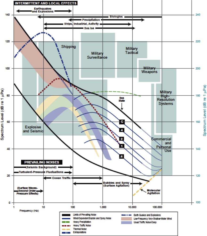
Composite of the ambient-noise spectra (after Wenz, 1962).
Caractéristiques du bruit ambiant sous-marin (d’après Wenz, 1962).
In the deep ocean, the profile of the sound speed affects the vertical and angular distribution of the ambient noise. Depending on this sound-speed profile, sound from surface sources can travel long distances without interacting with the ocean bottom. However, a receiver below a critical depth should sense less surface noise, as the propagation involves interactions with surface and/or bottom lossy boundaries.
In a range-independent ocean, the horizontal noise notch at depths where the speed of sound is less than the near-surface sound speed is predicted by Snell's law (Jensen et al., 1994). Here, we start from and assume a sound speed c = 1530 m/s at the surface and 1500 m/s at a receiver depth of 300 m. At the receiver, a horizontal ray (θ = 0) that is launched from the ocean surface would have an angle of about 11 degrees with respect to the horizontal, with all of the other rays arriving with greater vertical angles. These refraction effects thus result in a horizontal notch (i.e., an amplitude decay for a low grazing angle) in the vertical angular distribution of the ambient noise level. However, this horizontal notch is not always seen at shipping noise frequencies, as shipping tends to be concentrated in continental shelf regions. The consequent propagation down a continental slope will convert high-angle rays to lower angles at each bounce (Fig. 2a). Deep sound-channel shoaling effects also need to be considered, as these result in the same trend in angle conversion (Fig. 2b).
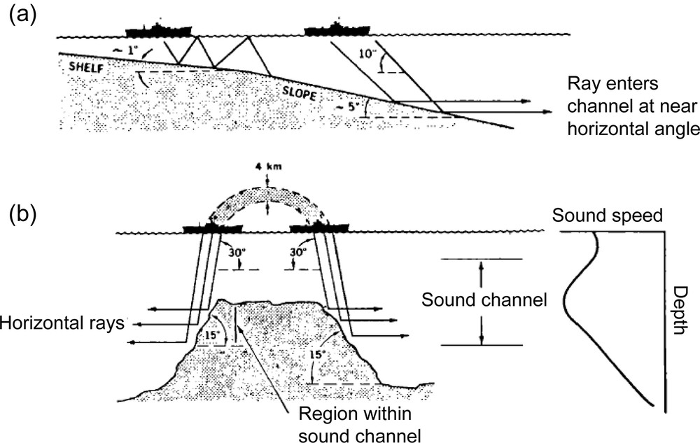
Effect of ocean bathymetry on shipping noise directivity. (a) In shallow water. (b) In deep water.
Influence de la bathymétrie sur la directivité du bruit des navires. (a) En zone côtière. (b) Dans l’océan profond.
The vertical directionality of ambient noise in shallow water has a simple environmental dependence (Kuperman and Ferla, 1985). This can be seen, for example, in a summer downward refracting profile, where the same discussion considered above leads to a horizontal noise notch (Fig. 3). However, in the winter, the vertical directionality of the noise from the surface will tend to be driven by the bottom properties. Thus, where the bottom is not very lossy, the surface sources that excite low-order modes can come from large distances (and hence large areas). As these paths are close to the horizontal, the noise will tend to have a stronger horizontal component. On the other hand, with a very lossy bottom, long-range propagating paths will be prevented from contributing to the noise field, and the noise will tend to be local, and subsequently vertical.
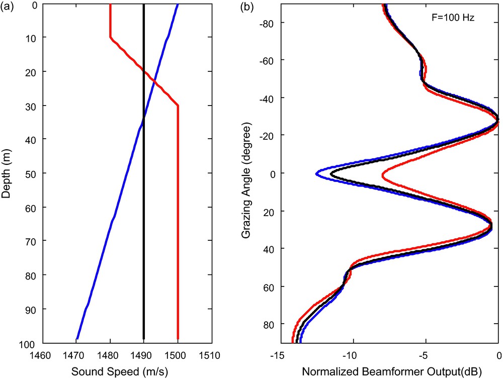
Computation of surface-noise directivity in a range-independent ocean waveguide. (a) Generic sound-speed profiles: uniform sound-speed profile (black, spring period), downward refracting sound-speed profile (blue, summer period) and surface duct sound-speed profile (red, winter period). (b) Vertical directionality at 100 Hz for each sound-speed profile. Negative angles are the upward direction from which we see the direct surface arrivals. The noise notch in the horizontal is typical of shallow waters, where the wave cannot simultaneously satisfy the surface and bottom boundary conditions (after Jensen et al., 1994).
Directivité spatiale du bruit de surface dans un guide d’onde sous-marin. (a) Exemples de profils de vitesse du son en fonction des saisons : uniforme au printemps (noir), à réfraction vers le fond en été (rouge), à réfraction vers la surface en hiver (bleu). (b) Directivité verticale du bruit à 100 Hz pour chacun de ces profils. Les angles négatifs pointent vers la surface (d’après Jensen et al., 1994).
Signal processing is common to many fields (Johnson and Dudgeon, 1993; Van Trees, 1971, 2002). Here, we focus on the application to underwater acoustics, as we will mainly concentrate on the spatial processing of pressure fields. However, we note that there is also a growing interest in the processing of vector fields, which include acoustic displacement, velocity or acceleration (D'Spain et al., 2006). The spatial sampling of a sound field is usually carried out with an array of distributed transducers; alternatively, a synthetic aperture array can be used, which is created by moving a single sensor through space. Spatial sampling is analogous to temporal sampling, whereby the sensor spacing value has the role of the sampling time. As a consequence, the Nyquist criterion requires that the sensor spacing is at least twice the spatial wavelength of the sound field measured. As the simplest example of array processing, there is phase shading in the frequency domain, where the bearing of a plane wave signal is searched for. This procedure is known as plane wave, or time-delay, beamforming.
Some of the general attributes of an array beamformer include:
- • the main lobe of the beamformer is defined as the “beamwidth”, the angular size of which depends on the array aperture and the acoustic frequency of the data;
- • the sidelobes are angular or wavenumber regions, where the array shows a relatively strong, but undesired response. In the worst situations, these sidelobes can sometimes be of comparable magnitude to the main lobe, although for a well-designed array, they are usually −20 dB or lower; i.e., the array response is less than 10% of the signal amplitude in the direction of the mainlobe;
- • instead of scanning through incident angles, the wavenumbers can be scanned through, as ; here, scanning through all of the possible kS values also results in the identification of non-physical angles that correspond to waves that are not propagating at the acoustic medium speed. These waves are sometimes referred to as virtual beams, and they are associated with array vibrations;
- • the array gain is defined as the decibel ratio of the signal-to-noise ratios of the array output to a single phone output. When the noise field is isotropic, the array gain (AG) is classically given by , where m is the number of array elements.
Among the numerous applications of array beamforming, array processing of low frequency ocean-generated noise has the potential to be very useful for the improvement of the body-wave tomography of the structure of the Earth. As an example, Fig. 4 illustrates the beamforming of seismic noise that was recorded in southern California, which reveals the P-wave that was generated by the distant storms in the open ocean.
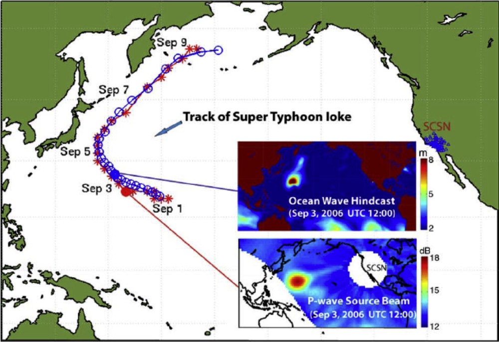
Tracks of the P-wave source regions (stars) and the super typhoon Ioke (circles). The track points of the peaks of source regions are derived from source beamforming using the Southern California Seismic Network seismic data (every 6 h, and limited by the 2° resolution). The best track of super typhoon Ioke is based on the observations and analysis of the Japan Meteorological Agency, available from [http://agora.ex.nii.ac.jp/digital-typhoon/]. The inserts show a map of the ocean wave hindcast and a map of the P-wave source region, sampled for September 3, 2006, UTC 12:00 (after Zhiang et al., 2010).
Suivi sismo-acoustique d’un typhon dans l’océan Pacifique Nord. Les étoiles rouges correspondent au résultat de beamforming sur les ondes P, effectué via le réseau sismique Southern California Seismic Network. Les ronds bleus correspondent au suivi du typhon Ioke par la Japan Meteorological Agency. Les inserts montrent une carte de l’intensité des vagues et une carte des sources des ondes P obtenues le 3 septembre 2006 (d’après Zhiang et al., 2010).
2 Cross-correlation of ocean ambient noise
Acousticians have used incoherent processing of ambient noise for small-scale imaging in the ocean (Buckingham et al., 1992; Makris et al., 1994) in the same way that optical imaging is achieved using incoherent light. On the other hand, in 2004, a collection of apparently incoherent ocean-noise sources was shown to be transformed into a coherent, large scale, imaging field (Roux et al., 2004). Indeed, every individual source of noise in the ocean (e.g., a collapsing bubble) generates an acoustic field that will be potentially coherent when it is received between two points after long-range propagation. However, this small coherent component at each receiver point will be buried in the spatially and temporally incoherent field that is produced by all of the widespread noise sources that are distributed over the ocean. Using ocean-noise data, it has been demonstrated experimentally that a long-time cross-correlation process can extract coherent wavefronts from the ambient noise without the support of any identifiable source. This means that noise can be used as a potential coherent source in the ocean, which leads to the concept of a self-imaging process.
As the instantaneous distribution of all of the mutually incoherent sources is extremely variable in space and time, it is difficult to identify a robust, space-time observable of the ocean noise. However, simple signal processing can reveal acoustic wavefronts that are strongly related to the time-domain Green's function (TDGF) between observation points.
These results originated from the research on helioseismology of Duvall (Duvall et al., 1993) and on earth seismology of Rickett and Claerbout (1999). The latter study was based on the following conjecture: “By cross-correlating noise traces recorded at two locations (…), we can construct the wavefield that would be recorded at one location if there was a source at the other”. This has since been experimentally confirmed: the ultrasonic research of (Lobkis and Weaver, 2001; Weaver and Lobkis, 2001) showed that the long-time, two-point correlation of random (Brownian motion) noise in an aluminum block cavity yields the deterministic TDGF between the two points.
As an analogy, the arrival-time structure of the two-point acoustic TDGF can be estimated in the ocean using ambient noise. In particular, the long-time correlation between a receiver and the elements of a vertical array of receivers yields a wavefront arrival structure at the array that is almost identical to the structure of the TDGF. The exception here is that the amplitudes of the individual wavefronts are shaded by the directionality of the noise sources. In the cases of both the cavity and the ocean, the Green's function emerges from the correlations that contain noise sources where the acoustic field passes through both of the receivers. The result from Weaver and Lobkis (2001) relies on noise sources that contribute to the construction of the TDGF that are three-dimensional (3-D), which leads to so-called modal equipartition in the cavity. However, there is no significant 3-D scattering in the frequency regime of the available data for the ocean environment considered here. Without the presence of identifiable events, only noise sources aligned along the line between the receivers will contribute over a long-time correlation (Roux et al., 2004; Sabra et al., 2005a).
2.1 Experimental demonstration with ocean data
The overall concept is summarized in Fig. 5, where ambient noise at two receivers, as array 1 and array 2, are pair-wise cross-correlated (Fig. 5b, c) (Roux et al., 2004). In Fig. 5d, e, this correlation is shown to be a function of delay time and space (the depths of the receivers in array 2), as is the TDGF between a position in array 1 and the receivers of array 2. The directivity pattern of the correlation process for a set of incoming angles is projected schematically on to the ocean surface (Fig. 5a). For each incident angle, the beamwidth between two receivers will depend on the central frequency and the bandwidth, and will correspond to a delay time in the correlation function. This directivity pattern demonstrates the contributions of the noise sources all over the ocean surface to the noise cross-correlation function. The noise sources inside the same space-time resolution cell in a particular direction will add together coherently, while noise sources from other beams will average out incoherently. In Fig. 5a, the two broader beams (the so-called end-fire beams) are aligned on the axis between the two arrays. Due to their size, these beams will provide a greater contribution to the noise-correlation function (NCF). For example, the two dashed lines in Fig. 5a show the coherent contribution from the surface-noise sources that travel through both of the receivers. Hence, the noise sources inside these end-fire beams will provide the residual time-averaged coherence between the two arrays. The actual noise-correlation process and the signal processing are carried out in the time domain. More precisely, the NCF C12(t) is measured using , where S1(t) and S2(t) are the ambient noise received on receivers 1 and 2 at time t. Note that the correlation processing requires data measurements that have a common clock time. The data that are available from the North Pacific Acoustic Laboratory program (NPAL, 2004) are used here, which were originally provided for ocean tomography purposes. These data correspond to different sets of 20-min simultaneous recordings of ambient noise on four vertical arrays that are filtered between 70 Hz and 130 Hz. Despite the obvious presence of shipping noise in this frequency bandwidth, high amplitude signals could not be identified in the spectrograms at the receivers. Fig. 5d shows an actual multi-day composite of three 20-min segments of simultaneous recordings of ocean data in this bandwidth (70–130 Hz). The wavefronts in the display obtained from the cross-correlation process are symmetric in time with respect to the zero time of the NCF, as the noise sources were distributed on both sides of the arrays. Note that there is no correlation between data that were not recorded at the same time (Fig. 5e). This confirms the hypothesis that required coherent wavefronts to be built up over time from the individual noise sources for which the acoustic field propagates through both of the receivers. Furthermore, using four coplanar arrays (Fig. 6a) has allowed us to measure the NCF with respect to the travel-time separation between one receiver in array 1 and all of the receivers in arrays 2, 3 and 4, as is shown in Fig. 6b–d. Note that in Fig. 6a and d, array 4 has twice as many elements as arrays 1–3. As can be seen from the correlation lag times, we have extracted wavefronts as they would propagate from a point source to ranges of 1700 m, 2400 m and 3500 m, (for arrays 1, 2 and 3, respectively). We also show that we recover similar wavefronts for the opposite direction, by correlating one receiver in array 4 with all of the receivers in arrays 1–3 (Fig. 6e–g). The sloping environment results in asymmetry between the two directions, i.e., the higher up the slope, the higher the reflection angle.
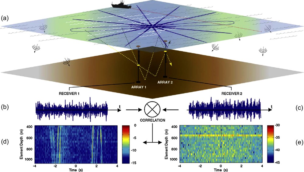
(a) Two arrays are depicted at a separation distance R. A schematic of the directivity pattern of the time-domain correlation process between two receivers on each array is projected on the ocean surface. Only a discrete set of lobes has been displayed, which corresponds to noise sources where the emission angle is −60°, −30°, 0°, 30°, 60° and 90°. Each angular lobe depends on the central frequency and bandwidth, and corresponds to a delay time in the correlation function. For the case of equally distributed ambient-noise sources, the broad end-fire directions will contribute coherently over time to the arrival times associated with the TDGF, while the contribution of the narrow off-axis sidelobes will average down. For the case of shipping noise, coherent wavefronts emerge only when there is sufficient intersection of the shipping paths with the end-fire beams. However, if there is a particular loud shipping event, it will dominate, so that either impractically long correlation times are needed, or discrete events should be filtered out. (b) and (c) The correlation process is carried out using time-domain ambient noise simultaneously recorded on two receivers, in arrays 1 and 2. (d) Spatial temporal representation of the wavefronts obtained from the correlation process between a receiver in array 1 at a depth of 500 m and all of the receivers in array 2 separated by a distance R = 2200 m. The arrival structure of the correlation function is composed of the direct path, surface-reflected, bottom-reflected, etc., as expected in the TDGF. The correlation function is plotted on a dB scale and normalized according to its maximum. (e) The same correlation processing is performed on data that have not been recorded at the same time on the two arrays. In (d) and (e), the horizontal and vertical axes correspond to the time axis of the cross-correlation function and receiver depth, respectively. The correlation functions are plotted on a dB scale and normalized according to the maximum of (d) (after Roux et al., 2004).
Approche schématique de la corrélation de bruit ambiant en mer. (a) Deux réseaux verticaux sont déployés à une distance R l’un de l’autre. Le diagramme de directivité associé au processus de corrélation entre les deux réseaux est projeté à la surface de l’océan pour un nombre discret d’ondes planes incidentes à −60°, −30°, 0°, 30°, 60° et 90°. (b) et (c) Le processus de corrélation est effectué dans le domaine temporel sur un intervalle de bruit enregistré simultanément sur deux récepteurs placés sur les réseaux 1 et 2. (d) Représentation spatiotemporelle des fronts d’onde issus du processus de corrélation entre un récepteur du réseau 1 à 500 m de profondeur et tous les récepteurs du réseau 2 à une distance R = 2200 m. La partie (d) est normalisée par rapport à son maximum et l’échelle de couleur est en dB. (e) Même représentation spatiotemporelle pour des fenêtres d’enregistrement non simultanées sur les récepteurs. La normalisation est effectuée par rapport au maximum obtenu en (d). En (d) et (e), les abscisses correspondent à l’axe des temps de la corrélation, les ordonnées à la profondeur des récepteurs sur le réseau 2 (d’après Roux et al., 2004).

The noise-extracted amplitude-shaded TDGF extracted from the NPAL data. (a) The array geometry indicating a sloping bottom. Note that array 4 has twice as many elements as arrays 1–3. (b–d) Time-domain correlation functions between a receiver at a depth of 500 m in array 1 and all of the receivers in the other arrays. Traveling wavefronts are clearly observed in the direction of the arrow, as if they emanated from the receiver in array 1. (e–g) Time-domain correlation functions between a receiver at a depth of 500 m in array 4 and all of the receivers in the other arrays. Here we see traveling wavefronts in the direction of the arrow, opposite to the case of (b–d), as if they emanated from the receiver in array 4. The wavefronts for this direction are more vertical because of the slope effect, further confirming the correct extraction of the arrival structure of the TDGF. In b–g, the horizontal and vertical axes correspond to the time axis of the correlation function and the receiver depth, respectively. The color scales are in dB (after Roux et al., 2004).
Représentation spatiotemporelle des fronts d’onde issus de la corrélation du bruit océanique entre des réseaux verticaux d’hydrophones. (a) La géométrie des réseaux indiquent un fond de l’océan en pente. Le réseau 4 comporte deux fois plus de récepteurs que les réseaux 1 à 3. (b–d) Représentation spatiotemporelle des corrélations pour un récepteur du réseau 1 à la profondeur de 500 m et l’ensemble des récepteurs des réseaux 2 à 4. (e–g) Représentation spatiotemporelle des corrélations pour un récepteur du réseau 4 à la profondeur de 500 m et l’ensemble des récepteurs des réseaux 3 à 1. De b–g, les abscisses correspondent à l’axe des temps de la corrélation, les ordonnées à la profondeur des récepteurs sur chaque réseau vertical (d’après Roux et al., 2004).
The basic difference between the Weaver cavity configuration (Weaver and Lobkis, 2001) and the ocean noise here is the 3-D reverberation physics of the cavity versus the 2-D ocean waveguide physics of the waves that are traveling in a horizontal direction. For the ocean, this means that a ray aligned along the receiver axis will pass through both of the receiver points by either reflection or refraction; however, if the ray has a horizontal component that is not along the horizontal line between the receivers, it cannot be reflected back to the second receiver. Such a ray cannot therefore contribute to the building-up of the coherent wavefronts between the receivers.
A separate experimental demonstration of the ocean-noise correlation process has been provided using data that were simultaneously recorded on two sono-buoys at a few hundred meters from each other in a shallow water environment (Roux et al., 2004). The noise was generated over 16 min in the 100 Hz to 300 Hz frequency range by a ship, the track of which is illustrated in Fig. 7a. The two 16-min-long-time-series can then be cross-correlated using different time windows (Fig. 7b–d). When the correlation is performed on a time series of 1 s (Fig. 7b), the ship track is clearly seen. If the length of the cross-correlated time series is increased to 10 s, and then up to 30 s (Fig. 7c–d, respectively), there is a tendency for the signature of the ship track to disappear, with the only signal that is left obtained when the ship crosses the end-fire main lobes (Fig. 7a). This signal has the different bottom and surface-reflected paths that are classically found in a shallow water environment. Obviously, we observe in Fig. 3b–d that the longer the correlation window, the higher the signal-to-noise ratio, as more acoustic sources participate coherently in the NCF. Assuming that the speed of the ship was constant along the track, this generates a uniform density of sources over time. For long-time windows, the signal-to-noise ratio of the correlation process can be defined as the ratio of the number of coherent versus incoherent sources inside the time window recording. Following the geometrical interpretation developed in Fig. 5, this ratio corresponds to the area enclosed from the end-fire beam to a non-end-fire beam. Although source motion typically degrades (due to the Doppler effect), the performance of wideband coherent processing schemes such as time-delay beamforming, it was demonstrated theoretically and numerically that the Green's function estimates extracted from ambient-noise cross-correlations are not significantly affected by the Doppler effect, even when considering supersonic sources under certain conditions (Sabra, 2010). The robustness towards the Doppler effect of this noise cross-correlation process primarily arises from its spatial directivity, as this emphasizes the contribution of the noise sources that cross the ray joining both of the receivers (i.e., the stationary-phase regions), where the differential Doppler effect between the stationary receivers is minimal.
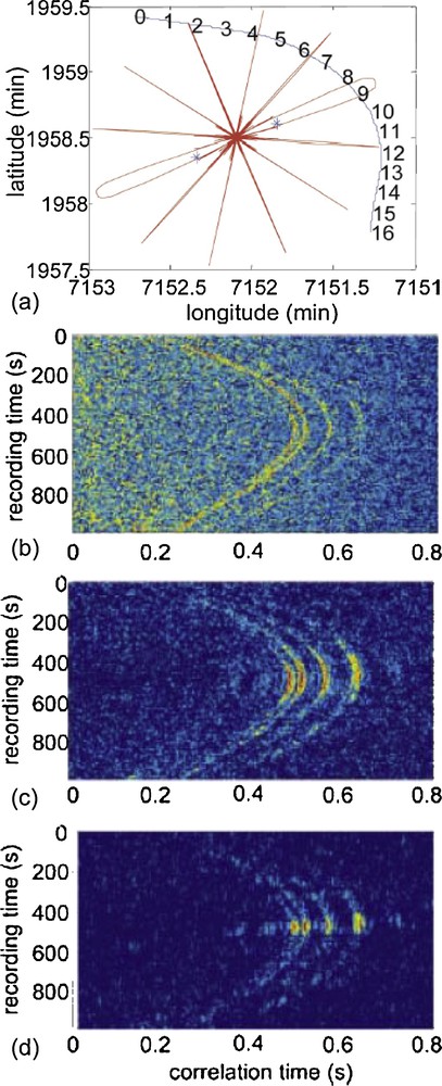
(a) Representation in latitude-longitude coordinates of the 16-min-long ship track (blue full line) with respect to the sono-buoy locations (blue ‘*’). The approximate distances between the sono-buoys is R ∼650 m. The average ship speed was constant, at 4.8 m/s. The directivity pattern of the time-domain cross-correlation process between the two sono-buoys is plotted in red. Only a discrete set of lobes has been displayed, which corresponds to noise sources where the emission angle is −60°, −30°, 0°, 30°, 60° and 90°. (b–d) Representation of the temporal evolution of the time-domain cross-correlation function between the two sono-buoys along the 16-min-long ship track. The horizontal and vertical axes correspond to the time axis of the correlation function and the ship position, respectively. The duration of the time windows on which the cross-correlation was performed is (b) 1 s, (c) 10 s and (d) 30 s. Each cross-correlation pattern is normalized according to its maximum. The color scales are in dB (after Roux et al., 2004).
Représentation spatiotemporelle de la corrélation mesurée en deux hydrophones en fonction de la position de la source dominante du bruit acoustique océanique. (a) Représentation latitude-longitude du trajet du bateau pendant les 16 minutes d’enregistrement de bruit ambiant (en bleu). La position des deux hydrophones est indiquée par les étoiles pour une distance approximative R ∼650 m. Le diagramme de directivité associé au processus de corrélation entre les deux hydrophones est représenté pour un nombre discret d’ondes planes incidentes à −60°, −30°, 0°, 30°, 60° and 90°. (b–d) Évolution temporelle de la corrélation entre les deux hydrophones durant les 16 minutes de suivi du trajet du bateau. Le temps de la corrélation est en abscisse et le temps d’enregistrement en ordonnée. La fenêtre de temps associé au processus de corrélation est de (b) 1 s, (c) 10 s et (d) 30 s. Chaque figure est normalisée par son maximum. L’échelle de couleur est en dB (d’après Roux et al., 2004).
2.2 Theoretical approach
The acoustic environment of the ocean is typically treated as a waveguide (Brekhovskikh, 1980; Jensen et al., 1994). As such, in its simplest form, the propagation between point 1 at depth z1 and point 2 at depth z2 that are separated by the horizontal range R (Fig. 4) is given by a normal mode expansion:
| (1) |
| (2) |
The wavefront structure of the Green's function arises from modes with similar group speeds constructively interfering over frequency; e.g., mathematically, the temporal wavefronts can be shown to emerge from a stationary-phase evaluation (Snieder, 2004) of Eq. (1).
On the assumption of a sheet of noise sources that is located at a given depth z’ close to the air-water interface, Kuperman and Ingenito (1980) obtained the following expression for the NCF:
| (3) |
| (4) |
shows the same wavefront structure as the two-point Green's functions, although the amplitude of the wavefronts will be different. Therefore, after the temporal averaging underlying Eq. (3), we conclude that we obtain coherent wavefronts from the ocean surface noise. However, these coherent wavefronts only constitute an approximation of the TDGF, as the excitation of each mode is weighted by dipole shading.
In Fig. 8, we confirm this theoretical approach with simulations using a spectral model (Schmidt and Jensen, 1985). This was performed for a shallow-water environment in the 50 to 150 Hz frequency bandwidth (Fig. 4). The time-domain NCF that is induced by the surface noise (Fig. 8a) is compared to the actual Green's function (Fig. 8b) between one source–receiver and an array of receivers. As expected, the same coherent wavefronts are seen, although the amplitude of the higher-order reflected paths is different. It has been shown that the relative amplitude of the noise-extracted reflected paths in shallow water is strongly dependent on the surface-noise frequency bandwidth and the depth of the surface-noise sheet, which is itself dependent on the wind conditions (Sabra et al., 2005a). Consistent with these results, the Green's function computed with a vertical dipole source instead of an omni-directional monopole excitation (Fig. 8c) shows an obvious similarity to the time-domain NCF.
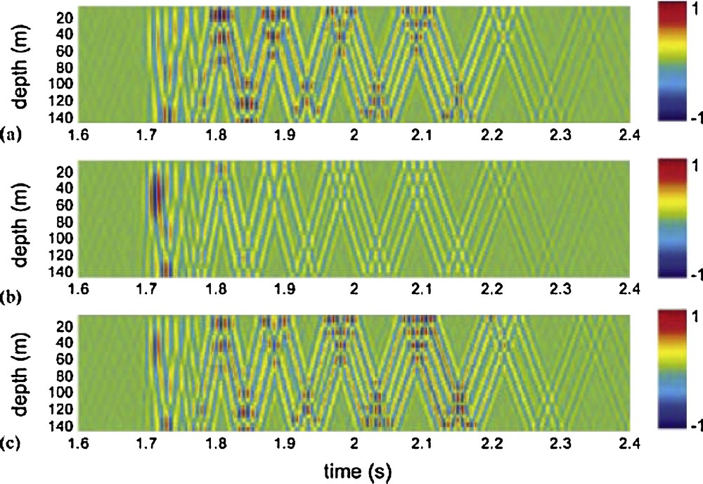
Spatiotemporal representation on a linear scale of (a) the time-domain cross-correlation function of surface noise computed between a receiver in z1 = 100 m and a receiver array at a distance R = 2,500 m in a 150-m-deep shallow water waveguide. The horizontal and vertical axes correspond to the time axis of the correlation function and the receiver depth, respectively. The surface noise sources are at depth z’ = 1 m. The sound-speed profile decreases linearly from 1,500 m/s at the surface to 1,480 m/s at the bottom. The bottom sound speed, density and attenuation are 1,800 m/s, 1,800 kg/m3 and 0.05 db/λ, respectively. (b) The TDGF computed between a source in z1 and a receiver array at the same distance R. (c) The TDGF computed in the same configuration as in (b) for a vertical dipole source at z1. The simulations were performed in the [50Hz-150 Hz] frequency bandwidth (after Roux et al., 2004).
Comparaison spatiotemporelle entre corrélation et fonction de Green dans un guide d’onde océanique pour une distribution de sources en surface via une approche numérique entre 50 et 150 Hz. Pour la corrélation, un récepteur est placé à z1 = 100 m de profondeur face à un réseau vertical de récepteurs qui couvrent toute la hauteur du guide d’onde (150 m) à une distance R = 2500 m. Le profil de vitesse décroît de 1500 m/s en surface à 1480 m/s au fond. La vitesse du son, la densité et l’atténuation dans le fond sont respectivement 1,800 m/s, 1,800 kg/m3 et 0,05 db/λ. (a) Corrélation temporelle entre le récepteur en z1 et le réseau vertical pour une distribution uniforme des sources de bruit à 1 m de profondeur sous la surface. (b) Fonction de Green obtenue sur le réseau vertical, pour une source ponctuelle en z1. (c) Fonction de Green obtenue sur le réseau vertical pour une source dipolaire en z1 (d’après Roux et al., 2004).
2.3 Practical issues related to the convergence time of the correlation process
The physical picture and the measurements presented above can be used to derive insight into the major components that govern the emergence rate of the coherent wavefronts for a homogeneous distribution of random sources. Considering two receivers separated by a distance R, the signal-to-noise ratio at the output of the NCF depends on three physical phenomena. First, this depends on the part of the signal that contributes to the correlation, as compared to the uncorrelated ambient noise, whether it is acoustic or electronic. The uncorrelated acoustic ambient noise corresponds to the field that passes through the two receivers. Secondly, the NCF is built from the contributions of the noise sources located in the end-fire beams versus the noise sources in the non-end-fire beams. Lastly, for a bandwidth Δf, the signal-to-noise ratio associated with a correlation process increases with the recording time, T, and is given by (Sabra et al., 2005b; Weaver and Lobkis, 2005). In any event, the total signal-to-noise ratio at the end of the correlation process is related to:
- • the time bandwidth product ;
- • the competition between the spatial gain of the correlator (which increases as ), the geometrical spreading in the propagation medium (which decreases as in a waveguide), and the attenuation factor (which decreases as );
- • an environmental factor (the expressions for local versus long-range contributions in Perkins et al. (1993), with the latter typically not known for an arbitrary location).
Without specific environmental knowledge, the rate of emergence of the TDGF is a measured parameter. For example, it is expected that this emergence rate will be different when considering either a non-isotropic azimuthal noise distribution or an isotropic noise environment instead. In practice, the successful implementation of the ambient-noise cross-correlation process to extract coherent wavefronts will be mainly determined by three factors: (1) the hardware configuration; (2) the choice of duration of the ambient-noise recordings used for the correlation process; and (3) the spatiotemporal distribution of the ambient-noise sources in the environment surrounding the receivers. The following discussion will suggest the optimal conditions for these three factors.
First, the noise cross-correlation process requires the use of time-synchronized receivers and the absence of any relative motion between them, to precisely determine the correlation arrival times. As moored or bottom-mounted arrays have a common time clock for each of the array-element recordings, this should provide an efficient hardware configuration. Additionally, transducers have a flat frequency response over a large bandwidth, which would allow the various arrival times in the NCF to be finely separated, even for noise-source depths that are relatively close to the sea surface.
Secondly, the choice of the recording time (Trec) determines the length of the cross-correlation window. This choice is driven by the need to record a sufficient number of uncorrelated noise events to be able to extract all of the different paths of the TDGF from the NCF. Thus, the Trec should be longer than two specific time factors: (1) the dispersion time of the sound channel (Tdisp), which corresponds to the temporal spreading of the TDGF between the two receivers (also referred to as the break time of the system); and (2) the statistical time, Tstat, which is defined as the average time required to converge towards a homogeneous distribution of spatially and temporally uncorrelated noise sources. Indeed, under the ergodic assumption, the noise events are considered to be realizations of a stationary stochastic process for which the corresponding time and ensemble averages of this process are equivalent. Any two particular noise events can have significant peaks in their cross-correlation functions due to the sidelobes and the other correlated parts of their waveforms. Thus, Tstat depends on the particular characteristics of the noise-source process, and it is usually an unknown parameter, although it can be estimated based on previous knowledge of the environment.
Furthermore, the formulation of the NCF is valid for a stationary environment. Thus, Trec should be smaller than the time scale of the fluctuations of the environment, Tfluc (e.g., considering currents, or tidal periods). Otherwise, an estimation of the NCF can be derived by averaging over several small correlation windows (such that Trec < Tfluc for each correlation window). However, in the case of the surface motion of the sea and a long averaging time, it is likely that Trec < Tfluc. However, the main effect of the motion of the sea surface might only be to prevent the emergence of acoustic paths associated with sea-surface reflections in the estimation of the TDGF extracted from the NCF. Overall, the practical use of the noise cross-correlation process needs to be optimal, as for the following order of the various time scales of the problem: Tdisp < Tstat < Trec < Tfluc.
Thirdly, and finally, a random homogeneous distribution of the uncorrelated noise point sources in space and time was assumed when the analytical expression of NCF in Eq. (3) was derived. The effect of the depth of the noise source, zs, distribution can be clearly identified and recognized from the cross-correlation measured. This approximation of the noise sources as being uncorrelated should hold for sufficiently long averaging times. However, the ability to extract a good estimate of the local Green's function from the NCF will depend on the spatial and temporal characteristics of the ambient-noise field. Indeed, the noise distribution might not be homogeneous in time or in space. For instance, a temporal inhomogeneous distribution can result from some loud noise events that occur at certain random times (e.g., a ship passing by, or a burst of sound). The influence of these loud events needs to be reduced, as they would otherwise bias the NCF. To this end, the noise recordings are frequency-filtered and their amplitude is clipped, in order to minimize the influence of isolated unique loud events prior to the computing of the cross-correlation function (Brooks and Gerstoft, 2009; Sabra et al., 2005c). In practice, this temporal and frequency equalization procedure needs to be adjusted and tuned so as to optimize the pre-processing of the ambient-noise recordings.
Additionally, the spatial anisotropic distribution of a noise source can be detrimental if there are no, or only a few, noise sources close to the end-fire direction of the two receivers. Indeed, on average, such noise sources contribute to the arrival times of the NCF that are not present in the TDGF between these two receivers. The bottom might also not be flat and it might not be equally absorbing in all spatial directions in the vicinity of a field test. This would thus lead to specific directionality of the noise field. Thus, a careful study of the spatiotemporal distributions of the noise sources is critical to be able to explain the performance of the noise cross-correlation process.
3 Application of noise correlation to ocean physics
3.1 Array synchronization and array-element localization
Coherent processing of data from an array of acoustic sensors (e.g., beamforming) requires an accurate positioning of the array elements. If the sensors are sampled by different data acquisition systems, then time synchronization between elements is also required, to compensate for the relative clock drift. Array-element localization is typically performed using: sensors embedded in the array (which can be acoustic or non-acoustic) (Lu et al., 2003; Wyeth, 1994); controlled active sources in the vicinity of the array (e.g., a towed source, acoustic pingers, an implosive source) (Dosso et al., 1998; Ferguson et al., 1992; Hodgkiss et al., 1996); or a distinctive opportunist source (e.g., a ship passing by the array) (Hodgkiss et al., 2003). These techniques rely on the detection of a specific beacon signal, and they involve additional equipment to be added to the acoustic array already deployed.
Ambient-noise cross-correlation is a promising alternative to the performing of array-element self-localization and self-synchronization on horizontal arrays. In particular, through the theory and data analysis in section II, it has been shown that the temporal structure of the ambient NCF between ocean sensors provides an estimate of their travel-time differences.
The data used in this analysis were recorded originally during the Adaptive Beach Monitoring experiment in May 1995 (ABM95), from 3.4 km off the coast of southern California. The ocean ambient-noise recordings were collected using two ocean-bottom hydrophone arrays, and they were processed in a frequency band of around 150 to 700 Hz (Fig. 9). ABM95 thus used ambient-noise data recordings from two bottom-mounted horizontal arrays located parallel to the shore in roughly 21 m of water. Each array comprised 64 hydrophones, and they recorded almost continuously for 2.5 weeks, at a sampling frequency of 1,500 Hz (Sabra et al., 2005c).
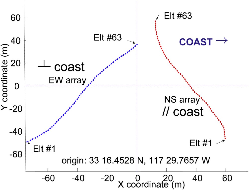
Geometry of the north-south and east-west bottom hydrophone arrays during the ABM 95 experiment. The locations of the first and last elements are indicated for both arrays (after Sabra et al., 2005c).
Géométrie des deux antennes horizontales d’hydrophones (nord-sud et est-ouest) utilisées durant l’expérience ABM 95 (d’après Sabra et al., 2005c).
Using only 11-min data blocks, two-sided coherent signals (traveling along the horizontal aperture of the array and corresponding to the direct arrival time of the TDGF) were extracted from the NCF (Fig. 10). The NCFs between several element pairs (within the same array or between the two arrays) were used for the array-element self-localization and self-synchronization (Fig. 11), as based on a nonlinear least squares algorithm. The data compared very well to previous reference measurements, within the uncertainty that was due to the limited bandwidth.

(a) Ambient-noise cross-correlation function, between element numbers 30 and 45 of the north-south array (Fig. 9). Eleven minutes of ambient-noise recordings was used (in the 350–700 Hz frequency band). Note that these elements were time-synchronized since the NCF is centered at τ = 0. (b) Stacked envelopes of the normalized cross-correlations for different pairs of the N = 64 elements, keeping element number 30 as the reference. The horizontal axis is the varying element index on the array (from 1 to 64). The vertical axis represents the positive and negative time delays of the NCF. The gray-scale color scheme corresponds to the amplitude of the NCF in decibels (0 to 20 dB). The NCF are normalized for each pair of elements (after Sabra et al., 2005c).
Représentation spatiotemporelle de la corrélation de bruit ambiant océanique sur une antenne horizontale d’hydrophones. (a) Corrélation temporelle entre les hydrophones 30 et 45 (Fig. 9) du réseau nord-sud pour 11 min d’enregistrement dans la bande 350–700 Hz. (b) Enveloppe des corrélations obtenue sur les N = 64 hydrophones par rapport à l’hydrophone 30. Le temps de la corrélation est en ordonnée, le numéro de l’hydrophone sur le réseau horizontal est en abscisse. La partie (b) est normalisée par son maximum. L’échelle de couleur est en dB (d’après Sabra et al., 2005c).

Ambient-noise cross-correlation function, between element number 63 of both the north-south and east-west arrays. Eleven min of ambient-noise recordings in the 350–700 Hz frequency band was used. The shifted symmetry line at t = 34:88 s (indicated by the thick dash-dotted line) corresponds to the unknown time offset between the ambient-noise recordings of the two arrays. The time interval between the two symmetric correlation peaks (as defined by the dashed lines) is twice the travel time between these two elements (Fig. 10a) (after Sabra et al., 2005c).
Corrélation de bruit ambiant océanique entre les hydrophones numéro 63 des deux réseaux horizontaux nord-sud et est-ouest dans la bande 350–700 Hz (d’après Sabra et al., 2005c).
Using the array-element locations estimated through noise-correlation processing, plane-wave beamforming was successfully achieved on a towed source in the vicinity of the arrays from the ABM95 data (Sabra et al., 2005c). Similar results were obtained recently in shallow-water areas where the tilt of vertical arrays was inverted in order to bring into focus marine mammal sound through matched-field processing (Thode et al., 2006). Another beamforming application was designed for diagnosis of the accidental switching of array elements during the autonomous deployment (Brooks et al., 2008).
3.2 Geo-acoustic inversion
The NCFs that resulted from these ABM95 data are also consistent with previous active acoustic experiments in this region, and they have allowed the extraction of individual environmental details. This is demonstrated by the identification of the critical angle at the water–sediment interface (Fried et al., 2008). The environment around the hydrophone arrays was measured and modeled using active geo-acoustic methods. Two nearby casts for conductivity, temperature and density provided the sound-speed profile for the water column. The measurements of the environment determined that this area was essentially range-independent.
Throughout the acquisition period, the hydrophones recorded significant biological activity, which was dominated by noise from the croaker fish (Sciaenidae) family. The ambient-noise levels were especially high at night, when the fish migrated from the surf zone out to the area where the hydrophones were located. As the noise field was dominated by biological activity within the water column (as opposed to waves breaking at the surface), this dataset is particularly useful for the extracting of the approximate TDGF. This is because the noise sources were volumetric, and thus a more accurate representation of the amplitude of the arrival structure can be expected, versus only surface-noise sources (Fig. 12a).
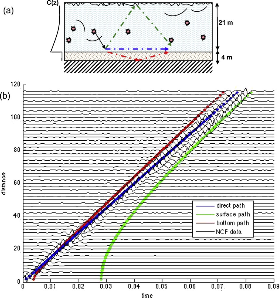
(a) Schematic of the ABM 95 shallow-water area. Based on conductivity, temperature and depth (CTD) cast measurements, a typical sound-speed profile shows a surface-mixed layer extending to 8 m in depth, with a negative gradient to approximately 21 m in water depth. This creates downward refracting acoustic propagation typical of summertime shallow-water environments. From geo-acoustic inversion results, the bottom is made of one 4-m sand layer (compressional speed, 1,607 ± 45 m/s) over a sandstone basement (compressional speed, 1,679 ± 15 m/s). The acoustic noise sources (croaker fish) are present in the whole water column. The direct, surface-reflected and bottom-reflected paths are represented by the blue, green and red arrows, respectively. (b) Spatially-averaged NCF result: the vertical axis is the distance between hydrophones, the horizontal axis is the correlation time. The structure of the time-versus-distance NCF reveals the complexity of the TDGF. The color lines correspond to travel-time predictions for the direct (blue line), surface-reflected (green line) and bottom-reflected (red line) paths. The environment used for travel time prediction is based on active acoustic measurements and inversions.
(a) Description schématique de l’expérience ABM 95. Le profil de vitesse C(z) est représenté sur la gauche. Une inversion géo-acoustique modélise le fond océanique par une couche de 4 m de sable (vitesse du son 1607 ± 45 m/s) reposant sur un substrat calcaire (vitesse du son 1679 ± 15 m/s). Différents trajets acoustiques entre deux hydrophones posés sur le fond sont représentés en bleu, vert et rouge. (b) Représentation spatiotemporelle de la corrélation de bruit. Le temps de la corrélation est en abscisse, la distance entre hydrophones est en ordonnée. Les lignes de couleurs bleue, verte et rouge correspondent aux temps de trajets théoriques pour le modèle et les trajets acoustiques obtenus en (a).
As the environment was relatively homogeneous throughout the time of the recordings, the different pairs of hydrophones that had the same separation between each other gave essentially the same response. The NCFs for the distinct pairs of hydrophones were then sorted according to this distance between the pairs. When these were stacked according to increasing separation distance between the hydrophones, the averaged NCF showed a time of arrival structure that was consistent with what would be expected from the theoretically calculated Green's function (Fig. 12b).
The environment for this simulation was taken from the geo-acoustic inversion of the same environment (McArthur, 2002). This comparison of the processed data with the predicted arrival times of the TDGF demonstrates that the cross-correlated data provide accurate times of arrival for signals traveling the given distances. Multiple returns are clearly visible in the NCF (and clearest at the greater distances), and they match the expected times of arrival of different ray paths between a source and receiver from the predicted Green's function.
In particular, the NCF shows the direct and surface reflection paths, where the surface reflection path is more visible for the shallower reflection angles (i.e., with a greater separation distance between the hydrophones). At distances more than 100 m, the surface reflection path begins to dominate over the direct path. At distances less than 40 m, approximately, the strength of the surface reflection path return dissipates, and a distinct second arrival is no longer detectable.
When isolated and plotted by distance, the amplitude ratio between the surface path arrival and the direct path arrival, the resulting curve shows a critical distance below which no surface arrivals are observed. This distance is then turned into a critical angle just above 20°, which is in agreement with the expected critical angle from the active geo-acoustic inversions (Jensen et al., 1994):
3.3 Bottom fathometer
The bottom fathometer (or sonic depth finder) was initially described by Siderius et al. (2006) and further developed by Gerstoft et al. (2008) and Siderius et al. (2010), and it is probably the most striking application of passive-noise processing in the ocean. The objective of the technique is to image the sea-bed layers using the cross-correlated ambient-noise field recorded by a drifting multi-element vertical array. This so-called passive fathometer technique exploits the naturally occurring acoustic sounds that are generated at the sea surface, primarily from breaking waves. The method is based on the cross-correlation of the incoming noise from the ocean surface with its echo from the sea-bed, which recovers travel times from significant sea-bed reflectors. Beamforming is used with a vertical array of hydrophones, to reduce the interference from the horizontally propagating noise, such that only the vertically propagating noise contributes coherently to the fathometer output. The initial developments used conventional beamforming, but significant improvements have been realized recently using non-linear adaptive beamforming (Fig. 13a) (Siderius et al., 2010).

(a) Adaptive beamforming passive fathometer results for the Boundary 2003 drifting array data (50–4000 Hz). The horizontal axis is the record number, which corresponds to the range as the array drifts (20 dB dynamic color scale). (b) Results from the data collected using a Uniboom active seismic system along approximately the same track as the array drift. The ping number on the horizontal axis corresponds to the range along the track (20 dB dynamic color scale) (after Siderius et al., 2010).
(a) Profilométrie du fond sous-marin obtenue par corrélation de bruit ambiant océanique associée à une technique de formation de voies adaptative sur une antenne verticale d’hydrophones dans la bande de fréquence (50–4000 Hz). L’échelle de couleur correspond à une dynamique de 20 dB. (b) Profilométrie du fond sous-marin obtenue par le système de sismique active Uniboom le long du même profil. L’échelle de couleur correspond à la même dynamique de 20 dB (d’après Siderius et al., 2010).
The ambient-noise data were recorded during the NATO Undersea Research Centre (NURC) Boundary 2003 experiment. The drifting array had 32 hydrophones with a separation of 0.18 m (design frequency of 4.2 kHz). The wind varied during the experiment, but on average it was about 7.5 m/s. The record numbers indicated in Fig. 13a (horizontal axis) correspond to the passive fathometer time trace of 90 s of noise averaging time. Therefore, each record number also equates to a range as the array drifted over time. The vertical axis in Fig. 13a gives the depths (in meters), which were converted from the two-way travel times using a sound speed of 1500 m/s. The passive fathometer results are in excellent agreement with the data collected using a Uniboom system (active sonar with a towed array) that was also used to measure the sub-bottom properties along the same track where the array drifted (Fig. 13b).
4 Conclusions
Although incoherent imaging with ambient noise has been demonstrated (which is commonly referred to as ‘acoustic daylight’ (Buckingham et al., 1992)), we have highlighted here the multiple potential uses of ambient-noise coherent imaging in ocean research. Applications for ambient-noise passive processing might emerge in the near future in research areas such as travel-time tomography, geo-acoustic inversion, and matched-field processing. The data shown in this review indicate the potential for noise-correlation processing for ocean imaging as a general concept. However, there still remains the need for the development of robust, consistent processing schemes that deal with ocean heterogeneities with sufficiently short emergence times. This would thus allow the production of data that have the space–time resolution necessary to provide useful information relating to the fluctuating ocean environment.