Signal and noise separation in time series of DORIS station coordinates using wavelet and singular spectrum analysis

Sofiane Khelifa; Salem Kahlouche; Mohamed Faouzi Belbachir

doi:10.1016/j.crte.2012.05.003

Internal geophysics (Geodesy)

Signal and noise separation in time series of DORIS station coordinates using wavelet and singular spectrum analysis
[Séparation du signal et du bruit dans les séries temporelles des coordonnées des stations DORIS en utilisant les ondelettes et l’analyse du spectre singulier]

Présenté par : Michel Petit

Sofiane Khelifa ¹ ; Salem Kahlouche ¹ ; Mohamed Faouzi Belbachir ²

¹ Centre of Space Techniques, PO Box 13, 31200 Arzew, Algeria
² University of Sciences and Technology of Oran-Mohamed Boudiaf (USTO-MB), PO Box 1505, 31000 Oran, Algeria

Comptes Rendus. Géoscience, Volume 344 (2012) no. 6-7, pp. 334-348.

Résumés

Anglais
Français

The aim of this article is to assess the noise in Doppler Orbitography and Radio-positioning Integrated by Satellite (DORIS) stations coordinate time series in order to better apprehend the spectral content of the non-linear station motion. In the frame of this work, we have used two different approaches to assess the noise, the wavelet transform in the frequency space, and the Singular Spectrum Analysis (SSA) in the phase space. The data used are the weekly solutions of coordinate residuals of 18 stations in STCD format (solution ign09wd01), computed by Institut géographique national/Jet Propulsion Laboratory (IGN, France/JPL, USA) using the GIPSY-OASIS II software package, referred to ITRF2005 and expressed in the local geodetic reference frame. The SSA has properly identified the non-linear trends and the seasonal signals (annual and semi-annual, 120, 59 and 20.3 days) in the analysed time series. The results show that the dominant signal present in the horizontal components (North and East) is mainly of a geophysical nature (plate tectonics) with a variance over more than 90% in most cases, and the remaining noise at 120 days was reduced in the ign09wd01 solution (w.r.t. the previous ign07wd01 solution). Using the wavelet transform method, we also identify, for the CADB station, a vertical discontinuity of 13 mm on 3 June 2008. For the noise level determination, both approaches converge to the same results. The standard deviation of the noise is in the range of 7–13, 8–24 and 7–14 mm in, respectively, North, East and Vertical components. The noise level is the highest in the east direction, probably related to the high orbit inclination of some DORIS satellites, and is lower in the high latitude stations which provide more observations from the DORIS satellites.

L’objectif de cet article est d’évaluer le bruit dans les coordonnées des stations Détermination d’Orbite et Radio-positionnement Intégrés par Satellite (DORIS) afin de mieux appréhender le contenu spectral du mouvement non linéaire des stations. Dans le cadre de ce travail, nous avons utilisé deux approches différentes pour évaluer le bruit, la transformée en ondelettes dans l’espace des fréquences, et l’analyse du spectre singulier (SSA) dans l’espace des phases. Les données utilisées sont les solutions hebdomadaires des résidus des coordonnées de 18 stations en format STCD (solution ign09wd01), calculées par l’Institut géographique national/Jet Propulsion Laboratory (IGN, France/JPL, États-Unis) en utilisant le logiciel GIPSY-OASIS II, référencées à l’ITRF2005 et exprimées dans le repère géodésique local. La SSA a bien identifié les tendances non linéaires et les signaux saisonniers (annuel et semi-annuel, 120, 59 et 20.3 jours) dans les séries temporelles analysées. Les résultats montrent que le signal primaire présent dans les composantes horizontales (Nord et Est) est principalement de nature géophysique (tectonique des plaques) avec une variance supérieure à 90 % dans la plupart des cas, et le bruit résiduel de 120 jours a été réduit dans la solution ign09wd01(relativement à la solution précédente ign07wd01). En utilisant la transformée en ondelettes, nous identifions également pour la station CADB une discontinuité verticale de 13 mm le 3 juin 2008. Pour la détermination du niveau de bruit, les deux approches convergent vers les mêmes résultats. La déviation standard du bruit est de l’ordre de 7–13, 8–24 et 7–14 mm dans les composantes Nord, Est et Verticale, respectivement. Le niveau du bruit est plus élevé dans la direction Est, probablement lié à la haute inclinaison d’orbite de certains satellites DORIS, et il est faible dans les stations de haute latitude, qui fournissent plus d’observations à partir des satellites DORIS.

Métadonnées

Reçu le : 2011-10-13
Accepté le : 2012-05-27
Publié le : 2012-06-01

DOI : 10.1016/j.crte.2012.05.003

Keywords: DORIS, Time series analysis, Wavelet, Singular Spectrum Analysis, De-noising
Mot clés : DORIS, Analyse des séries temporelles, Ondelette, Analyse du spectre singulier, Dé-bruitage

Affiliations des auteurs :

Sofiane Khelifa ¹ ; Salem Kahlouche ¹ ; Mohamed Faouzi Belbachir ²

¹ Centre of Space Techniques, PO Box 13, 31200 Arzew, Algeria
² University of Sciences and Technology of Oran-Mohamed Boudiaf (USTO-MB), PO Box 1505, 31000 Oran, Algeria

@article{CRGEOS_2012__344_6-7_334_0,
     author = {Sofiane Khelifa and Salem Kahlouche and Mohamed Faouzi Belbachir},
     title = {Signal and noise separation in time series of {DORIS} station coordinates using wavelet and singular spectrum analysis},
     journal = {Comptes Rendus. G\'eoscience},
     pages = {334--348},
     publisher = {Elsevier},
     volume = {344},
     number = {6-7},
     year = {2012},
     doi = {10.1016/j.crte.2012.05.003},
     language = {en},
}

TY  - JOUR
AU  - Sofiane Khelifa
AU  - Salem Kahlouche
AU  - Mohamed Faouzi Belbachir
TI  - Signal and noise separation in time series of DORIS station coordinates using wavelet and singular spectrum analysis
JO  - Comptes Rendus. Géoscience
PY  - 2012
SP  - 334
EP  - 348
VL  - 344
IS  - 6-7
PB  - Elsevier
DO  - 10.1016/j.crte.2012.05.003
LA  - en
ID  - CRGEOS_2012__344_6-7_334_0
ER  -

%0 Journal Article
%A Sofiane Khelifa
%A Salem Kahlouche
%A Mohamed Faouzi Belbachir
%T Signal and noise separation in time series of DORIS station coordinates using wavelet and singular spectrum analysis
%J Comptes Rendus. Géoscience
%D 2012
%P 334-348
%V 344
%N 6-7
%I Elsevier
%R 10.1016/j.crte.2012.05.003
%G en
%F CRGEOS_2012__344_6-7_334_0

Sofiane Khelifa; Salem Kahlouche; Mohamed Faouzi Belbachir. Signal and noise separation in time series of DORIS station coordinates using wavelet and singular spectrum analysis. Comptes Rendus. Géoscience, Volume 344 (2012) no. 6-7, pp. 334-348. doi : 10.1016/j.crte.2012.05.003. https://comptes-rendus.academie-sciences.fr/geoscience/articles/10.1016/j.crte.2012.05.003/

Version originale du texte intégral

1 Introduction

The developments of space geodesy have allowed the establishment of global observing systems. Doppler Orbitography and Radio-positioning Integrated by Satellite (DORIS) (Barlier, 2005; Willis et al., 2006) is one of these systems, as Satellite Laser Ranging (SLR) (Pearlman et al., 2002), Very Long Baseline Interferometry (VLBI) (Schlueter and Behrend, 2007; Schlueter et al., 2002) and Global Positioning System (GPS) (Beutler et al., 1999; Dow et al., 2009). The large number of measurements collected by these systems permit today to represent the displacement of the ground stations in terms of coordinates time series.

The analysis of coordinate time series allows one to better apprehend the temporal variability of the physical phenomena (deformations of the Earth's crust, mass transfers, geodynamic local phenomena, etc.). Pioneering studies were undertaken in the late 1990s in the GPS system by King et al. (1995), Langbein and Johnson (1997), Zhang et al. (1997), Mao et al. (1999) and Williams et al. (2004). These authors implemented standard statistical methods, e.g. spectral density or maximum likelihood estimation (MLE), separately on the North, East and Up components (NEU) of the time series, in order to determine the noise characterization (type and level) of each component. In the DORIS system, to characterize the type and level of noise in weekly coordinates (NEU) time series, Le Bail (2006) and Feissel-Vernier et al. (2007) have used the Allan variance (Allan, 1966), while Williams and Willis (2006) have employed the MLE method. The main advantage of MLE method is to determine the type of noise (white noise, flicker noise and random walk noise) and its amplitude. However, its limitation is that several combinations should be tested, since the method does not identify directly the type of noise (iterative process), while the Allan variance can directly and rapidly detect the type and level of noise, but requires that the time series should be regular (gaps should be filled) and stationary (elimination of trend and all periodic components). This study is a contribution to these methodological developments. We apply the wavelet and the Singular Spectrum Analysis (SSA) methods on the weekly position time series of DORIS stations to extract the noise from the signal, in order to provide certain information useful to later geodynamic interpretations such as the trend, seasonal components and residual noise contained in these time series.

The wavelet and SSA are well-known methods already applied in a variety of disciplines (geophysics, meteorology, biosciences, economics, etc.). The wavelet technique (Daubechies, 1992) permits to study the signal at different resolutions using functions (wavelets) well localized in both physical space (time) and spectral space (frequency), generated from each other by translation and dilation which is well suited for investigating the temporal evolution of periodic and transient signals. The SSA (Broomhead and King, 1986) technique permits to decompose the original time series into the sum of a small number of independent and interpretable components such as a slowly varying trend, oscillatory components and a structureless noise.

The article is organized as follows. For the convenience of the reader we briefly recall the wavelet and SSA approaches in Sections 2 and 3, respectively. Section 4 describes the data analysed in this study. Results and discussion are reported in Section 5, and finally the conclusion is drawn in Section 6.

2 Wavelet transform

A wavelet is a function ψ(t) of L² (R) (L²(R): continuous functions of real variable and square integrable) which satisfies the following properties (Daubechies, 1992; Mallat, 1999; Ranta, 2003):

• zero mean: $\int_{- \infty}^{+ \infty} ψ (t) dt = 0$ ;
• unitary norm: $\int_{- \infty}^{+ \infty} |ψ {(t)}^{2}| dt = 1$ ;
• centred around t = 0.

We introduce the factor of translation (or position) u and the scale factor (or dilatation) s; therefore, we define a family of functions ψ_u,s called wavelets, deriving all of the mother wavelet ψ, such as:

ψ_{u, s} (t) = \frac{1}{\sqrt{s}} ψ (\frac{t - u}{s}) u, s \in R; s \neq 0

(1)

The Wavelet transform can be defined as the projection of the signal X(t) on the basis of wavelet functions ψ_u,s:

WT (u, s) = < X, Ψ_{u, s} > = \int_{- \infty}^{+ \infty} X (t) {\bar{ψ}}_{u, s} (t) d t

(2)

where u and s denote the translation and scale factor, respectively, and

{\bar{ψ}}_{u, s}

denotes the complex conjugate of ψ_u,s.

The original signal can be reconstructed from its wavelet coefficients WT(u,s) with consideration that the wavelet ψ checks the admissibility condition (Daubechies, 1992; Holschneider, 1998):

C_{ψ} = \int_{0}^{+ \infty} \frac{{|F T (ψ (t))|}^{2}}{t} d t < + \infty

(3)

where FT is the Fourier Transform.

The inverse wavelet transform uses the standardization coefficient C_ψ given by:

X (t) = \frac{1}{C_{ψ}} \int_{u \in ℜ} \int_{s > 0} W T (u, s) ψ_{u, s} (t) d u \frac{d s}{s^{2}}

(4)

2.1 De-noising steps

The majority of wavelet algorithms use a decimated discrete decomposition of the signal (Daubechies, 1992; Holschneider, 1998; Mallat, 1989). This decomposition has the characteristic to be orthogonal and to concentrate information in some great wavelet coefficients. The de-noising idea is to conserve only the greatest coefficients and put the others (corresponding to the noise) at zero before reconstruction of the signal.

Assume that the observed data vector X = [X₁, X₂,…, X_N]^t is given by:

X_{t} = S_{t} + R_{t}, t = 1,2,..., N

(5)

where S_t is the true signal and R_t is Gaussian white noise centred independent and identically distributed (iid) of variance σ², such as

R_{t} \overset{i i d}{\sim} N (0, σ^{2})

Let W(.) and W⁻¹(.) denote the forward and inverse discrete wavelet transform operators. Let D(., λ) denote the de-noising operator with threshold λ.

The de-noising procedure proceeds in three steps:

• decomposition: choose a wavelet and choose a level l. Compute the wavelet decomposition of the signal X at level l; W = W(X);
• thresholding of the wavelet coefficients: Z = D(W,λ);
• reconstruction: from the coefficient thresholding, one reconstructs the signal: S = W⁻¹(Z).

2.2 Strategies of thresholding

Donoho and Johnstone (Donoho, 1995; Donoho and Johnstone, 1994) propose two types of thresholding functions denoted T_λ:

• hard thresholding: $T_{λ}^{H a r d} (W) = \{\begin{array}{c} W i f |W| > λ \\ 0 i f |W| \leq λ \end{array}$
• soft thresholding: $T_{λ}^{S o f t} (W) = \{\begin{array}{c} W - λ i f W \geq λ \\ W + λ i f W \leq - λ \\ 0 i f |W| \leq λ \end{array}$

where W are wavelet coefficients and λ is threshold value (λ > 0).

2.3 Determination of the threshold

The thresholding method suggested in this work is the VisuShrink (Donoho and Johnstone, 1994) based on the mean square error minimization. This method proposes a universal threshold λ, which depends only on the number of measurements N and the noise variance σ². It is used when the noise is independent and identically distributed according to a centred normal law; its value is given by:

λ = \hat{σ} \sqrt{2 log (N)}

(6)

The noise variance σ² can be calculated by a robust estimator from the median Med of the absolute values of the wavelet coefficients at the first level of decomposition as follows:

\hat{σ} = \frac{Med}{0.6745}

(7)

The factor 0.6745 is selected from a calibration with Gaussian distribution.

3 Singular spectrum analysis

The SSA method allows one to extract significant components from time series (trends, periodic signals and noise) (Broomhead and King, 1986; Ghil et al., 2002; Vautard et al., 1992). The method is based on the computation of the eigenvalues and the eigenvectors of a covariance matrix C formed from the time series {X_t, t = 1,…, N} and the reconstruction of this time series based on a number of selected eigenvectors associated with the significant eigenvalues of the covariance matrix. The algorithm of SSA includes the following steps.

3.1 Step (1): choice of the embedding dimension M

The time series {X_t, t = 1,…, N} is embedded into a vector space of dimension M. The embedding dimension M must be sufficiently long to include the assumed periodicity of the time series without exceeding half of the length of the time series.

3.2 Step (2): computation of the M × M covariance matrix C

Computation of the M × M covariance matrix C given by:

C = \frac{1}{N^{'}} D^{t} D D = (\begin{array}{c} X_{1} & X_{2} & \dots & X_{M} \\ X_{2} & X_{3} & \dots & X_{M + 1} \\ ⋮ & ⋮ & ⋱ & ⋮ \\ X_{N - M + 1} & X_{N - M + 2} & \dots & X_{N} \end{array})

(8)

where N is the length of the time series and N′ = N – M + 1.

3.3 Step (3): study of the eigenvalues of the covariance matrix C

The M eigenvalues of the covariance matrix C once determined are ordered by decreasing value. Each eigenvalue λ_k gives the Partial Variance (PV), given by Eq. (9), of the original time series in the direction specified by the corresponding eigenvectors E_k.

PV (k) = \frac{λ_{k}}{\sum_{k = 1}^{M} λ_{k}}

(9)

If we arrange and plot the ordered eigenvalues, one can often distinguish an initial steep slope, representing the true signal, and a (more or less) “flat floor” representing the noise (Vautard and Ghil, 1989). Thus, the theory of the SSA allows one to conclude that (Le Bail, 2004):

• the signal has a trend if the diagram contains an isolated eigenvalue;
• the signal is periodic if there are two close eigenvalues that have the same dominant frequency;
• the small eigenvalues constitute the noise of the signal.

3.4 Step (4): projection of the original time series onto the k-th eigenvectors and its reconstruction

By the eigenvectors {E_k, 1 ≤ k ≤ M}, called Empirical Orthogonal Functions (EOFs), we can construct the time series of length N′ (N′ = N – M + 1) given by:

A_{k} (t) = \sum_{j = 1}^{M} X (t + j - 1) E_{k, j} t = 1,..., N^{'},

(10)

where E_k,j represents the value of the jth line corresponding to kth eigenvector.

A_k(t) called the k-th principal component (PC). It represents the projection of the original time series onto the k-th EOF (with 1 ≤ k≤ M). The sum of the power spectral of the PC is identical to the power spectral of the time series X(t) (Vautard et al., 1992) and therefore, we can study separately the spectral contribution of the various components.

The PCs, however, have length N′, not N, and do not contain phase information. In order to extend the time series to length N, it is necessary to choose a subset of EOFs on which the reconstruction is based, the associated PCs are combined to form the partial reconstruction R_к(t) of the original time series X(t).

R_{k} (t) = (\begin{array}{c} \frac{1}{t} \sum_{k \in k} \sum_{j = 1}^{t} A_{k} (t - j + 1) E_{k, j}, 1 \leq t \leq M - 1 \\ \frac{1}{M} \sum_{k \in k} \sum_{j = 1}^{M} A_{k} (t - j + 1) E_{k, j}, M \leq t \leq N^{'} \\ \frac{1}{N - t + 1} \sum_{k \in k} \sum_{j = t - N + M}^{M} A_{k} (t - j + 1) E_{k, j}, N^{'} + 1 \leq t \leq N \end{array})

(11)

These series R_к(t) of length N are called the reconstructed components (RCs). They have the important property of preserving the phase of the time series; therefore, X(t) and R_к(t) can be superimposed. No information is lost in the reconstruction process, since the sum of all individual RCs gives back the original time series.

4 Data used

For this study, we have used the weekly position residuals of DORIS stations (solution ign09wd01) in STation Coordinate Difference (STCD) format (Noll and Soudarin, 2006), available on the International DORIS Service (IDS) (Willis et al., 2010a) website at http://ids-doris.org/network/ids-station-series.html.

The data are provided by Institut géographique national/Jet Propulsion Laboratory (IGN, France/JPL, USA) (Willis et al., 2010b), using the GIPSY-OASIS II software package (Zumberge et al., 1997), referred to ITRF2005 (Altamimi et al., 2007) and expressed in the local geodetic reference frame (dN: North component, dE: East component and dH: Vertical component). The observing satellites are SPOT series from 2 to 5, TOPEX/Poseidon, Envisat, Jason-2 and Cryosat-2. The Jason-1 data are not used in the ign09wd01 solution, as these data are affected by a large error related to the extreme and unexpected sensitivity of the on-board receiver to radiation over the South Atlantic Anomaly (Lemoine and Capdeville, 2006; Willis et al., 2004). This DORIS/IGN solution is the latest one from this group. It was prepared in for the IDS combination (Valette et al., 2010) in view of ITRF2008 (Altamimi et al., 2011) and includes the latest available data processing strategies to mitigate errors in solar radiation pressure models (Gobinddass et al., 2009a, 2009b) as well as high-frequency errors in atmospheric drag corrections (Gobinddass et al., 2010).

We should point out that DORIS time series in STCD format are also provided by two other analysis centres: Institute of Astronomy Russian Academy of sciences (INASAN) (Kuzin et al., 2010) and Laboratoire d’études en géophysique et océanographie spatiales/Collecte et localisation par Satellite (LEGOS/CLS) (Soudarin and Cretaux, 2006). We chose to use the IGN/GPL solution (ign09wd01) because it is the most recent one and because it is regularly updated (on average every week).

The time series selected in this application, as seen in Table 1 and Fig. 1, are the coordinate residuals of 18 stations with data gaps less than 3 months and their observing period is longer than 4 years. For this study, we had to remove some outliers, which are not included in the tolerance interval, given by:

[- (μ - μ_{α} σ), (μ - μ_{α} σ)]

where μ, σ are the average and standard deviation of the time series, respectively, and μ_α is fractile factor of the normal distribution provided by the usual statistical tables. The value taken is equal to 2.5. Also note that the data gaps are filled by a linear interpolation.

Acronym	Site	Country	Latitude (°)	Longitude (°)	Data span
ADFB	Terre Adélie	Antarctica (French base)	–66.67	140.00	2008.2–2011.3
ARFB	Arequipa	Peru	–16.47	–71.50	2006.6–2011.3
CADB	Cachoeira Paulista	Brazil	–22.68	–45.00	2004.3–2011.3
DIOB	Dionysos	Greece	38.01	23.93	2006.4–2011.3
DJIB	Djibouti	Djibouti	11.53	42.85	2006.6–2011.3
HBMB	Hartebeesthoek	South Africa	–25.88	27.70	2007.2–2011.3
HEMB	St-Helena	UK (South Atlantic Ocean)	–15.95	–5.67	2003.2–2011.3
KOLB	Kauai	USA (Hawaii)	22.12	–159.67	2002.9–2011.3
LICB	Libreville	Gabon	0.35	9.67	2005.9–2011.3
MIAB	Miami	USA	25.73	–80.17	2005.2–2011.3
REZB	Reykjavik	Iceland	64.15	–21.98	2004.8–2011.3
RIQB	Rio Grande	Argentina	–53.78	–67.75	2008.3–2011.3
ROUB	Rothera	Antarctica (UK base)	–67.57	–68.12	2007.9–2011.1
SANB	Santiago	Chile	–33.15	–70.67	2001.5–2011.3
SYPB	Syowa	Antarctica (Japanese base)	–69.00	39.58	1999.3–2011.3
TLSB	Toulouse	France	43.55	1.48	2007.5–2011.3
YASB	Yarragadee	Australia	–29.01	115.35	2003.9–2011.3
YEMB	Yellowknife	Canada	62.48	–114.48	2007.6–2011.3

Fig. 1
Map of the 18 sites selected in this study.
Carte des 18 sites sélectionnés dans cette étude.

Table 2 shows the percentages of outliers and interpolated points (data gaps and values considered as aberrant) relative to the total number of points (number of observations). We remark that the time series ADFB, HBMB and YEMB present the largest proportions of data gaps (relatively to their observation period) over the periods respectively: (2010.69–2010.88), (2010.75–2010.94) and (2010.75–2010.94). In general, the cause of these data gaps could be related to equipment problem affecting either the data quality (oscillator problem) or the physical location of the antenna (antenna tilt), as discussed in Willis et al. (2009). It could also be linked to a lesser amount of DORIS data in the first weeks after first data availability or to a local geophysical phenomenon (earthquake, landslide, etc.). We note that the difference between the percentages of outliers and interpolated points in the North component of ARFB station is due to the elimination of the two first points deemed aberrant and therefore not taken into account in the interpolation of data gaps. We note the same thing for the components North and Vertical of DIOB station. Consequently, the first point has been removed from each component.

Station	Series (mm)	Obs. nbr.	Gaps (week)	Perc. outliers	Perc. interp.	Station	Series (mm)	Obs. nbr.	Gaps (week)	Perc. outliers	Perc. interp.
ADFB	dN	152	9	2.0	11.8	MIAB	dN	320	0	0.6	0.6
dE	1.3	11.2	dE	0.3	0.3
dH	3.3	13.2	dH	1.9	1.9

ARFB	dN	246	0	1.2	0.4	REZB	dN	340	0	0	0
dE	2.9	2.9	dE	0	0
dH	2.9	2.9	dH	0.6	0.6

CADB	dN	345	9	0.3	7.3	RIQB	dN	160	0	0.6	0.6
dE	1.2	7.8	dE	0.6	0.6
dH	0	7.0	dH	0.6	0.6

DIOB	dN	257	0	0.4	0	ROUB	dN	169	0	0.6	0.6
dE	1.2	1.2	dE	0.6	0.6
dH	2.0	1.6	dH	3.0	3.0

DJIB	dN	249	0	0	0	SANB	dN	506	7	0.4	1.8
dE	0.4	0.4	dE	0.6	2.0
dH	2.0	2.0	dH	1.6	3.0

HBMB	dN	190	9	0.5	15.3	SYPB	dN	626	2	1.8	2.4
dE	2.1	16.8	dE	2.2	2.9
dH	1.6	16.3	dH	2.6	3.2

HEMB	dN	420	2	0	3.1	TLSB	dN	201	0	0.5	0.5
dE	0	3.1	dE	0.5	0.5
dH	1.0	4.1	dH	1.5	1.5

KOLB	dN	441	1	0	0.2	YASB	dN	387	1	0	0.3
dE	0	0.2	dE	0	0.3
dH	1.6	1.8	dH	1.8	1.3

LICB	dN	274	9	0.4	3.7	YEMB	dN	175	5	1.1	14.3
dE	0.4	3.7	dE	0.6	13.7
dH	1.1	4.4	dH	1.7	14.9

5 Results and discussion

5.1 Trend

As previously mentioned, the SSA technique requires, a priori, the choice of the embedding dimension M which depends on the periodicity of the time series without exceeding half of the length of the time series. In this application, we have taken arbitrarily M = 52 weeks which corresponds to one year.

Fig. 2 represents the diagrams of the logarithms of the 52 eigenvalues for the components (North: dN, East: dE and Vertical: dH) of stations at high latitude. The first eigenvalue, which is clearly visible from the other remaining values, indicates the signature of a dominant trend represented by the Reconstructed Component RC 1 as seen in Fig. 3.

Fig. 2
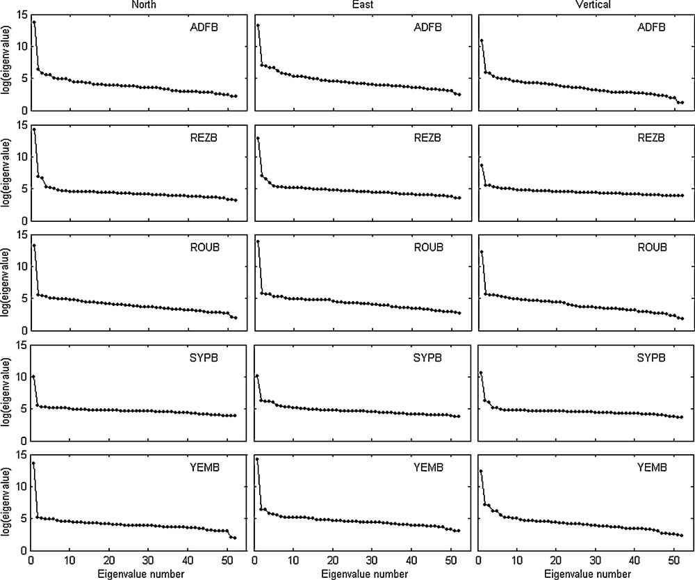
Diagrams of the 52 eigenvalues for the components (North, East and Vertical) of stations at high latitude.
Diagrammes des 52 valeurs propres pour les composantes (Nord, Est et Verticale) des stations de haute latitude.

Fig. 3
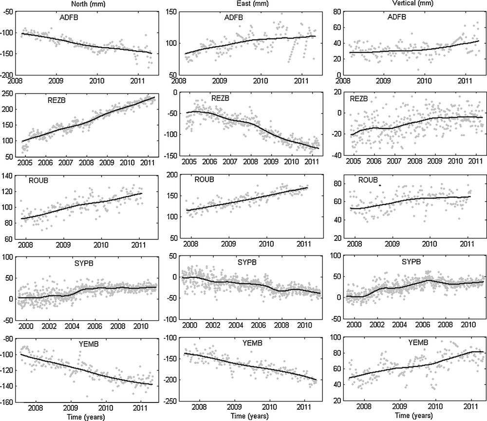
Superposition of the original components (North, East and Vertical) of stations at high latitude with their non-linear trend (reconstructed component RC1).
Superposition des composantes originales (Nord, Est et Verticale) des stations de haute latitude, avec leur tendance non linéaire (composante reconstruite RC1).

The results provided in Table 3 show that the partial variance of trend in the most horizontal components (North and East) of studied stations explains over 90% of the total signal and it is more important compared to the Vertical component. Globally, the horizontal displacements of the stations are usually due to plate tectonics (Argus et al., 2010) and the vertical displacements may be due to local subsidence or postglacial rebound (King et al., 2010; Willis et al., 2009).

Station	Series (mm)	Partial variance	Slope (mm/yr)	GEODVEL velocity	Station	Series (mm)	Partial variance	Slope (mm/yr)	GEODVEL velocity
ADFB	dN	99.59	–14.95 ± 0.15	–12.16	MIAB	dN	88.37	2.05 ± 0.09	1.94
dE	98.54	11.02 ± 0.15	7.79	dE	96.62	–12.70 ± 0.07	–10.26
dH	94.90	2.77 ± 0.10		dH	14.67	1.61 ± 0.03

ARFB	dN	89.57	6.07 ± 0.22	10.34	REZB	dN	99.65	21.63 ± 0.07	19.28
dE	76.89	11.35 ± 0.29	–2.24	dE	98.29	–15.28 ± 0.13	–9.23
dH	20.15	6.50 ± 0.21		dH	54.46	2.64 ± 0.04

CADB	dN	98.09	15.15 ± 0.07	11.94	RIQB	dN	99.55	16.36 ± 0.09	10.69
dE	70.85	–4.78 ± 0.22	–3.49	dE	77.00	6.26 ± 0.07	1.87
dH	80.18	16.65 ± 0.58		dH	87.40	0.11 ± 0.14

DIOB	dN	98.65	–14.41 ± 0.05	^a	ROUB	dN	99.40	9.96 ± 0.07	10.45
dE	94.69	5.78 ± 0.06	^a	dE	99.57	17.13 ± 0.04	13.78
dH	11.33	–1.78 ± 0.06		dH	98.11	4.65 ± 0.11

DJIB	dN	99.68	16.49 ± 0.06	15.15	SANB	dN	93.77	7.01 ± 0.46	10.42
dE	99.78	31.61 ± 0.07	23.62	dE	82.27	2.49 ± 0.87	–0.24
dH	91.21	1.25 ± 0.02		dH	53.76	–0.67 ± 0.04

HBMB	dN	99.30	16.50 ± 0.09	17.28	SYPB	dN	78.56	2.63 ± 0.04	2.77
dE	98.56	15.34 ± 0.19	17.30	dE	79.11	–3.18 ± 0.03	–3.52
dH	71.03	2.17 ± 0.07		dH	88.77	3.04 ± 0.07

HEMB	dN	99.36	20.18 ± 0.08	17.66	TLSB	dN	99.52	15.56 ± 0.07	15.50
dE	99.07	21.13 ± 0.05	22.46	dE	99.46	14.86 ± 0.04	19.26
dH	45.02	4.06 ± 0.07		dH	9.73	1.72 ± 0.04

KOLB	dN	99.74	33.16 ± 0.07	34.15	YASB	dN	99.93	57.01 ± 0.08	57.06
dE	99.90	–61.09 ± 0.09	–62.98	dE	99.83	39.88 ± 0.08	38.61
dH	15.46	0.92 ± 0.06		dH	82.43	0.57 ± 0.05

LICB	dN	99.66	15.86 ± 0.05	18.25	YEMB	dN	99.61	–10.50 ± 0.05	–10.51
dE	99.12	21.02 ± 0.08	22.04	dE	99.58	–16.63 ± 0.07	–17.24
dH	46.97	6.20 ± 0.10		dH	97.21	8.23 ± 0.10

^a The Aegean Sea plate (location of DIOB station) is not included in the model GEODVEL2010.

Our results (Table 3) show that the velocities values of the North and East components for most DORIS stations are consistent with those of GEODVEL (for GEODesy VELocity) model (Argus et al., 2010) provided by UNAVCO at http://www.unavco.org/community_science/science-support/crustal_motion/dxdt/model.html. We note a particularity in the velocity values of Arequipa (ARFB) and Rio Grande (RIQB) stations. For Arequipa, this is due to post-seismic relaxation after the June 23 2001 (magnitude 8.1) earthquake (Willis et al., 2009). For Rio Grande, this can be explained that this site is moving east relative to the South America plate at a significant velocity (2.2 ± 1.3 mm/yr) (Argus at al., 2010), which is consistent with the hypothesis (Smalley et al., 2003) that left-lateral shear across a wide east-striking zone in Patagonia causes the region several tens of kilometres north of the Magallenes-Fagano fault to be moving east relative to the interior of the South America plate. However, the GEODVEL model does not solve for the motion of all tectonic plates; the small Aegean Sea plate is not included in this model. For this reason, the horizontal velocities of Dionysos station (DIOB), which is located on the Aegean Sea plate, are not provided in Table 3.

However, the low partial variances in the Vertical component for the stations ARFB, DIOB, KOLB, MIAB and TLSB compared to other stations can be explained by the fact that these sites are experiencing a small vertical deformation as a result of Glacial Isostatic Adjustment (GIA). In the ICE-5G (VM2) model (Peltier, 2004), ARFB station has a predicted vertical rate of 0.8 mm/yr, DIOB 0.1 mm/yr, KOLB –0.3 mm/yr, MIAB –1.5 mm/yr and TLSB –0.2 mm/yr. Furthermore, the high velocity in the Vertical component of the station CADB is particularly significant; which can be explained by the fact that the position and velocity solutions for this station could be affected by errors related to the South Atlantic Anomaly (SAA) effect on SPOT-5 (Bock et al., 2010; Stepanek et al., 2010), especially as this station is located just in the centre of the SAA and at least for stations located just close to the SAA as ARFB, HEMB and SANB. Another possibility is also that this station presents a positive vertical discontinuity around mid 2008 that has not been previously detected by any DORIS group. Using the wavelet transform (multiresolution analysis) (Khelifa et al., 2012), the approximation signal at level 5 (Fig. 4) shows a discontinuity of 13 mm and a change in velocity on 3 June 2008. To identify this discontinuity, we have used the wavelet of Daubechies “db2” which is more appropriate for this kind of application (Mallat and Hwang, 1992). YEMB results present the largest amplitude for the vertical velocity (8.23 mm/yr). This value is very close to the value predicted by the ICE-5G (VM2) model (i.e. 8.3 mm/yr).

Fig. 4
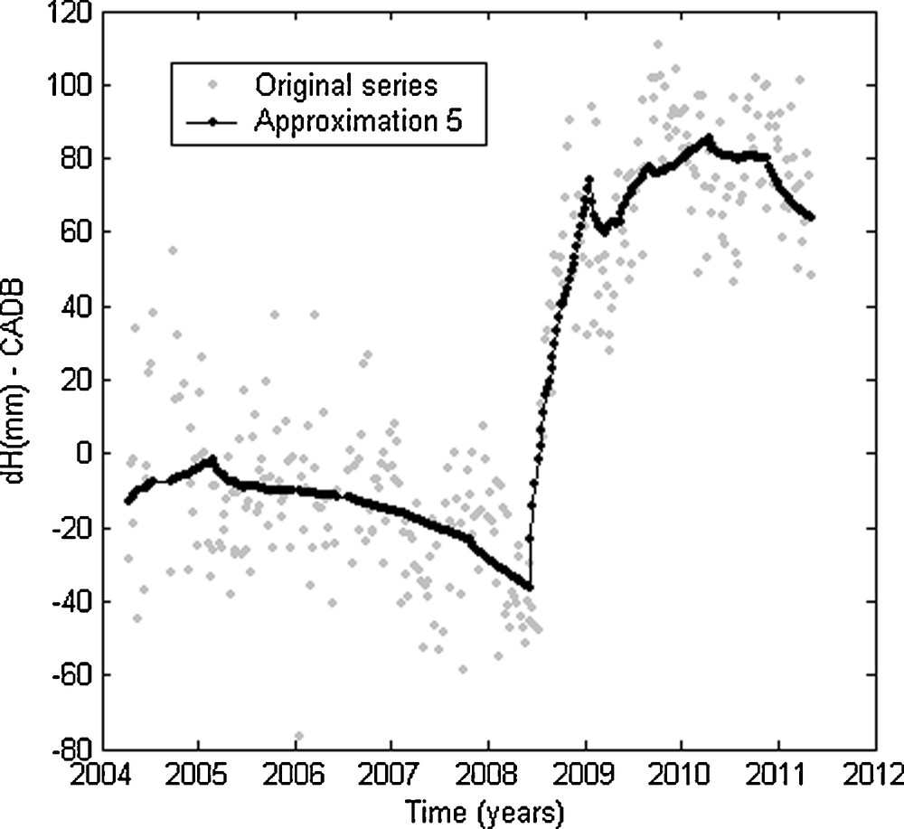
Highlighted by the signal of approximation 5 (Khelifa et al., 2012) a discontinuity of 13 mm in the Vertical component of CADB station, on 3 June 2008.
Mise en évidence par le signal d’approximation 5 (Khelifa et al., 2012) d’une discontinuité de 13 mm dans la composante Verticale de la station CADB, le 3 juin 2008.

5.2 Seasonal signals

The main skill of SSA is its ability to automatically and easily detect the dominant periodic signals in the time series; near equality of a great eigenvalues pair is associated with a dominant seasonal signal activity. Figs. 5–7 show a few examples of seasonal signals contained in the studied time series and their periodicities identified by periodogram. The most important peaks on the periodogram indicate the values of the periodicities contained in the signal such as annual and semi-annual signals, 117, 59, and 20.3 days. In Fig. 5, the reconstructed component RC 2-3 of the North component of HEMB station, based on the second and third EOFs (eigenvectors), reveals a clear annual signal with a partial variance of 0.20%, and the reconstructed components RC 4-5 and RC 6-7 in the East component illustrate, respectively, a periodic signals of 59 and 20.3 days with a partial variance of 0.10% and 0.08%, respectively. Fig. 6 reveals an evident semi-annual signal contained in the Vertical component of SANB station with a partial variance of 3.45%, and the Fig. 7 shows a seasonal signal of 117 days in the Vertical component of ADFB and TLSB stations with a partial variance of 1.23% and 5.01%, respectively.

Fig. 5
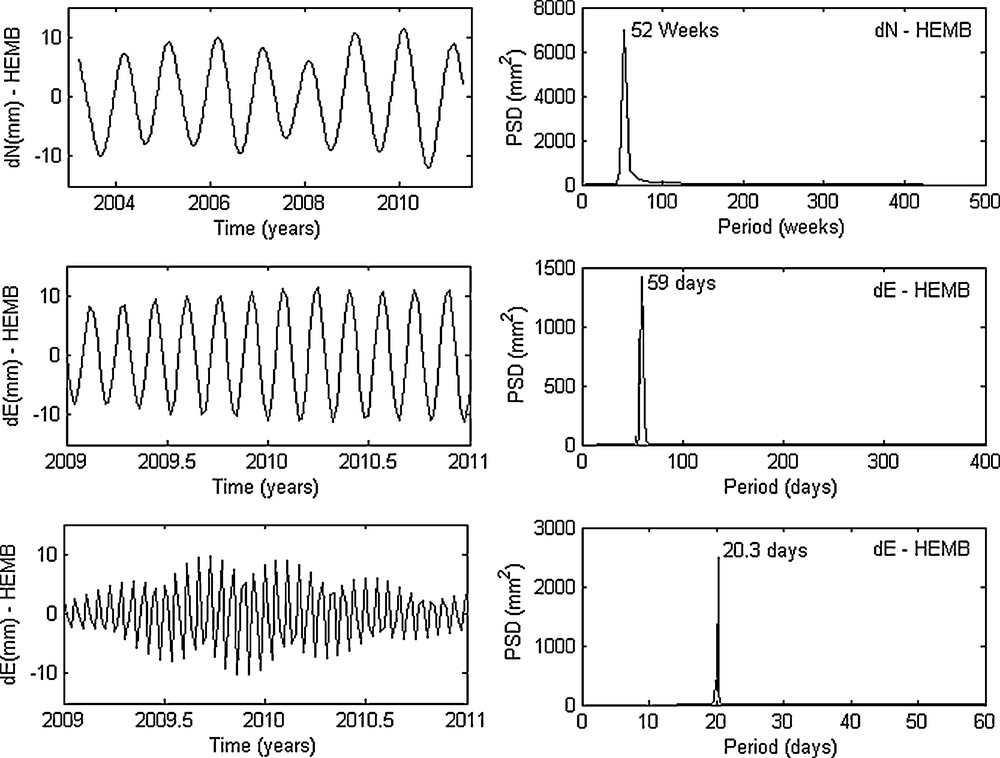
Seasonal signals in the North and East components of HEMB station with their Power Spectral Density PSD (periodogram). The annual signal in the North component is represented by the reconstructed component RC 2-3, and the seasonal signals of 59 and 20.3 days in the East component are represented respectively by RC 4-5 and RC 6-7 over the last two years (2009–2011).
Signaux saisonniers dans les composantes Nord et Est de la station HEMB, avec leur densité spectrale de puissance DSP (périodogramme). Le signal annuel dans la composante Nord est représenté par la composante reconstruite RC 2-3, et les signaux saisonniers de 59 et 20,3 jours dans la composante Est sont représentés respectivement par RC 4-5 et RC 6-7 au cours des deux dernières années (2009–2011).

Fig. 6
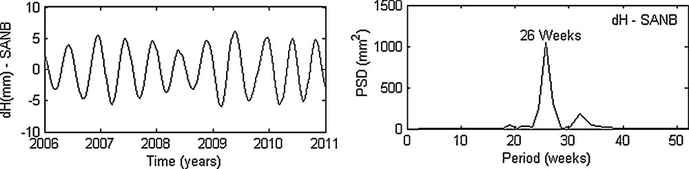
The semi-annual signal (represented by the reconstructed component RC 4-5) and its periodogram in the Vertical component of SANB station over the last five years (2006–2011).
Le signal semi-annuel (représenté par la composante reconstruite RC 4-5) et son périodogramme dans la composante Verticale de la station SANB au cours des cinq dernières années (2006–2011).

Fig. 7
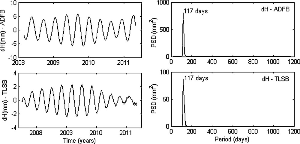
The seasonal signal of 117 days and its periodogram in the Vertical component of ADFB (represented by the reconstructed component RC 2-3) and TLSB (represented by the reconstructed component RC 5) stations.
Le signal saisonnier de 117 jours et son périodogramme dans la composante Verticale de la station ADFB (représentés par la composante reconstruite RC 2-3) et de la station TLSB (représenté par la composante reconstruite RC 5).

The annual and semi-annual errors and the term of 117 days were previously detected by several authors (Le Bail, 2006; Mangiarotti et al., 2001; Williams and Willis, 2006). The annual periodicity may be connected to the draconitic period of the sun-synchronous SPOT satellites (Gobinddass et al., 2009b) or to un-modelled effects in atmospheric density models used for satellite drag correction (Gobinddass et al., 2010), while the semi-annual periodicity could probably be related to the atmosphere perturbation (Stepanek et al., 2010). However, the periodicity of 117 days is the draconitic period of the TOPEX satellite (Gobinddass et al., 2009a, 2009b), while the periodicity of 20.3 days could be connected to the hydrological phenomena and atmospheric loading (Williams and Willis, 2006), and the periodicity of 59 days could be associated to the 117.3 days (–3.0679 degree/day) period of the angle between the TOPEX orbital plane and the sun (Williams and Willis, 2006).

We should point out that the error of 120 days was supposed to be removed or at least mitigated in the ign09wd01 solution (Gobinddass et al., 2009a, 2009b), as the latest ign09wd01 solution is the result of a computation which takes into account a better strategy for the computation of the solar radiation pressure. For this reason, we have tried to check the noise remaining at 120 days in the analysed solution (ign09wd01) and to compare it with that in the previous solution (ign07wd01). For example, this error was detected in the ign03wd01 solution by (Bessissi et al., 2009) using the wavelets in the Vertical component of SYPB station. In the frame of this work, this error was also detected using the SSA on the same component (Fig. 8) in the ign07wd01 solution, but not in the case of ign09wd01 solution. The same error was also detected in the North component of CADB station (Fig. 8) in the ign07wd01 solution, but not in the case of ign09wd01 solution. Taking the stations which have a common period of observation longer than 4 years for both solutions (ign07wd01 and ign09wd01), we have found this error in the two solutions in the Vertical component of KOLB, East component of SYPB and North component of YASB (Fig. 9). The results show that the variance of this error, in respectively ign07wd01 and ign09wd01 solutions, was decreased from 3.27% to 2.90% for KOLB, 7.42% to 4.83% for SYPB and 0.04% to 0.01% for YASB. The amplitude of this error, computed as the average of amplitudes of this periodicity over the same observation period for the two solutions, is also decreased; passing for the solution ign07wd01 to the solution ign09wd01 from respectively: 3.2 to 1.6 mm for KOLB, 5.6 to 4.8 mm for SYPB and 3.0 to 1.9 mm for YASB. However, our results are in agreement with the results derived by (Gobinddass et al., 2009a, 2009b) which stipulate that the new solution ign09wd01 is an improvement over the previous ign07wd01 solution.

Fig. 8
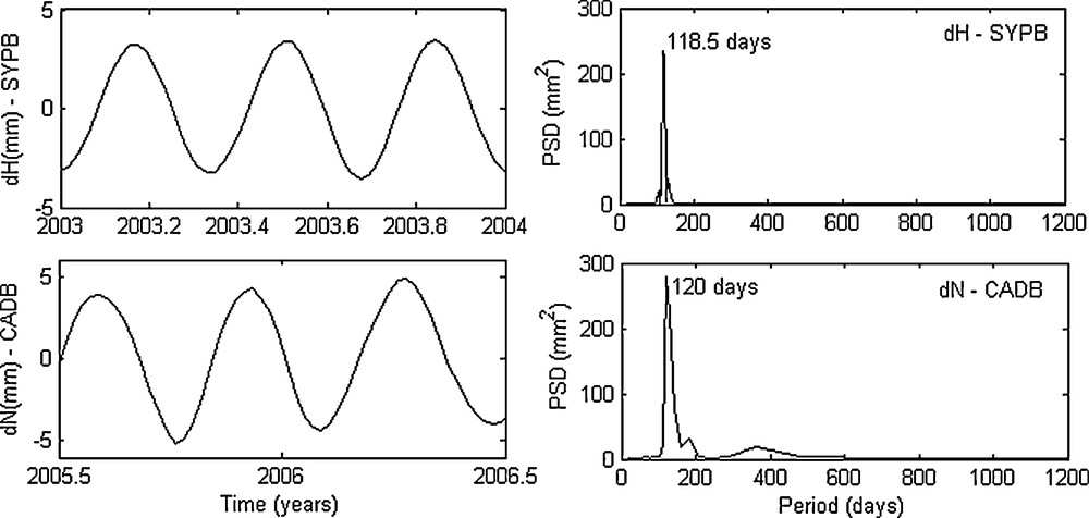
The seasonal signal of 120 days and its periodogram in the Vertical component of SYPB station (represented by the reconstructed component RC 5) and the North component of CADB station (represented by the reconstructed component RC 5-6) for the ign07wd01 solution.
Le signal saisonnier de 120 jours et son périodogramme dans la composante Verticale de la station SYPB (représentés par la composante reconstruite RC 5) et la composante Nord de la station CADB (représentés par la composante reconstruite RC 5-6) pour la solution ign07wd01.

Fig. 9
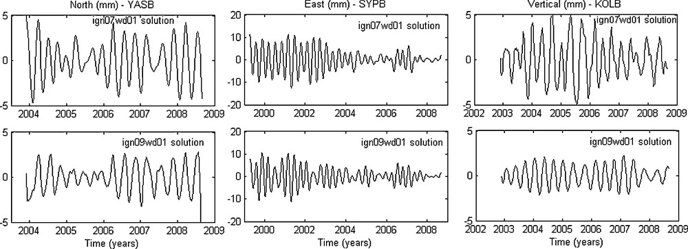
The seasonal signal of 120 days in the components: North of YASB station (represented by the reconstructed component RC 4), East of SYPB (represented by the reconstructed component RC 3-4) and Vertical of KOLB (represented by the reconstructed component RC 3-4) for the two solutions ign07wd01 and ign09wd01.
Le signal saisonnier de 120 jours dans les composantes : Nord de la station YASB (représenté par la composante reconstruite RC 4), Est de SYPB (représenté par la composante reconstruite RC 3-4) et Verticale de KOLB (représenté par la composante reconstruite RC 3-4) pour les deux solutions ign07wd01 et ign09wd01.

5.3 Noise determined by Singular Spectrum Analysis and wavelet

The SSA allows one to assess the noise affecting the time series by extracting the reconstructed components from the initial time series. In the diagram of the eigenvalues, the noise is characterized by much lower values that form a flat floor or a mild slope (Pike et al., 1984; Vautard and Ghil, 1989). In our case, the noise is extracted from the original components (North, East and Vertical) after removing their reconstructed components (de-noised time series) based on the first EOFs associated to the largest eigenvalues which correspond to trends (linear or non-linear) and various oscillatory components.

The critical point in wavelet analysis is the choice of optimal wavelet function which depends on the kind of applications (Meyer, 1992). In our application, we have used the Meyer wavelet as in Bessissi et al. (2009). The wavelet coefficients used in this analysis are calculated from a decomposition of the signal at level 4 using the VisuShrink method with soft thresholding.

Figs. 10 and 11 represent the noise and the de-noised components (dN, dE and dH) for the stations at high latitude determined by SSA and wavelet, respectively. The obtained results show that the de-noised components determined by wavelet are more regular and smooth relatively to those determined by SSA which is probably related to the continuous character of soft thresholding function.

Fig. 10
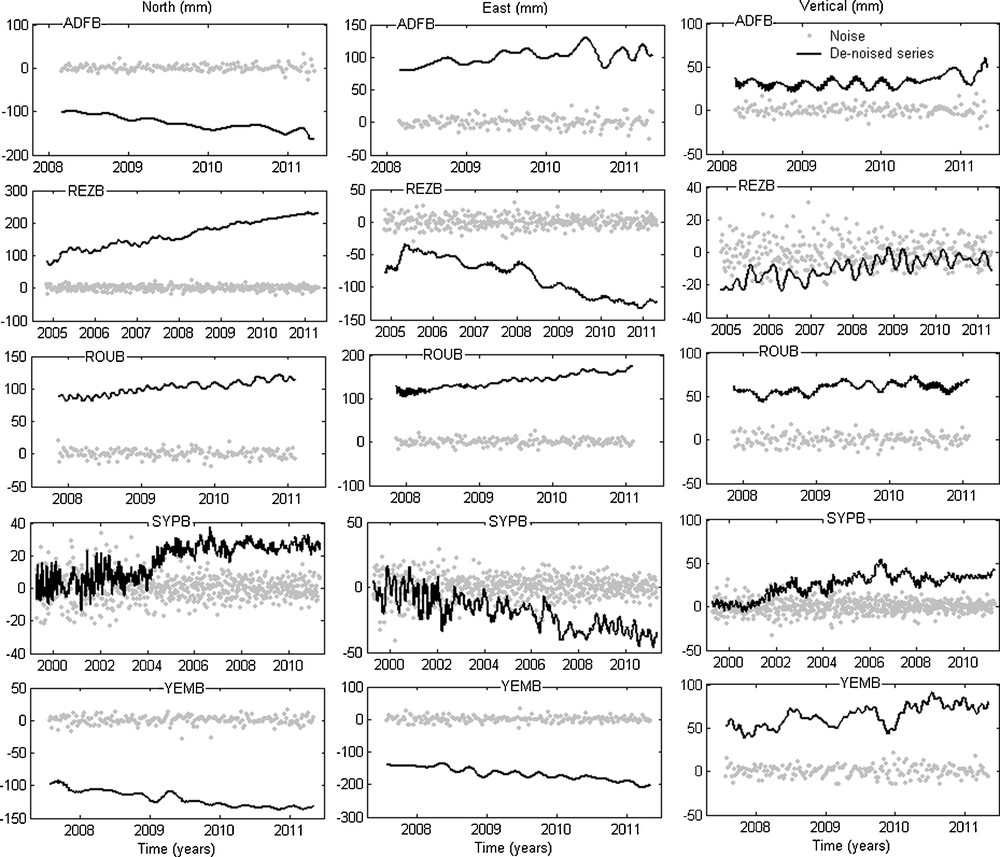
The noise and the de-noised components (North, East and Vertical) determined by Singular Spectrum Analysis for the stations at high latitude.
Le bruit et les composantes dé-bruitées (Nord, Est et Verticale) déterminés par l’analyse du spectre singulier pour les stations de haute latitude.

Fig. 11
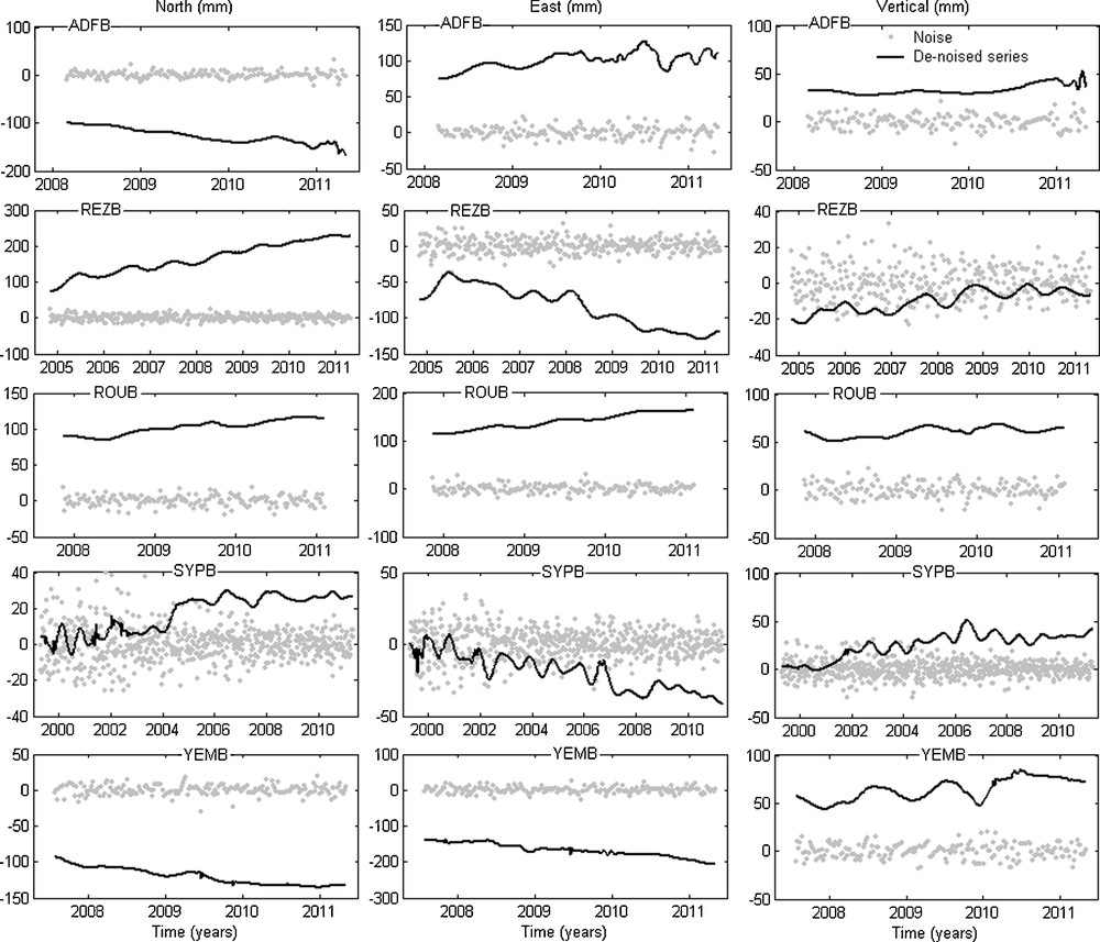
The noise and the de-noised components (North, East and Vertical) determined by wavelet for the stations at high latitude.
Le bruit et les composantes dé-bruitées (Nord, Est et Verticale) déterminés par ondelettes pour les stations de haute latitude.

Table 4 shows that the standard deviation (STD) of the noise determined by SSA in the North, East and Vertical components ranges between 7–13, 8–24 and 7–14 mm respectively, and that determined by wavelet is about 7–14, 8–27 and 7–16 mm, respectively. Therefore, the both techniques give almost the same results in term of standard deviation.

Station	Technique	STD – North (mm)	STD – East (mm)	STD – Vertical (mm)
ADFB	Wavelet	7.2	8.2	7.1
SSA	7.2	8.2	5.7

ARFB	Wavelet	14.3	27.6	15.8
SSA	11.9	24.0	14.9

CADB	Wavelet	13.6	22.2	15.5
SSA	13.1	19.5	13.2

DIOB	Wavelet	10.3	11.8	9.2
SSA	9.0	11.0	7.4

DJIB	Wavelet	8.0	13.0	9.4
SSA	7.6	12.2	8.8

HBMB	Wavelet	9.7	15.4	14.0
SSA	9.8	13.0	11.6

HEMB	Wavelet	9.9	15.8	10.4
SSA	9.4	14.9	9.1

KOLB	Wavelet	10.2	12.2	8.9
SSA	9.5	11.4	7.7

LICB	Wavelet	9.1	15.1	10.5
SSA	8.5	14.5	9.1

MIAB	Wavelet	10.6	14.9	8.4
SSA	10.2	14.2	7.6

REZB	Wavelet	8.1	9.9	9.1
SSA	7.3	8.8	8.3

RIQB	Wavelet	8.4	12.7	10.0
SSA	7.5	9.9	7.8

ROUB	Wavelet	7.2	8.6	7.6
SSA	6.4	7.3	6.5

SANB	Wavelet	12.4	21.7	12.5
SSA	11.6	20.6	10.8

SYPB	Wavelet	9.8	10.2	9.0
SSA	8.3	8.6	7.9

TLSB	Wavelet	8.4	12.3	9.0
SSA	7.5	10.4	7.4

YASB	Wavelet	10.4	12.0	7.8
SSA	9.2	10.8	6.9

YEMB	Wavelet	7.0	8.8	7.6
SSA	6.4	8.5	6.5

The East component is generally less well determined than the two others; most DORIS satellites have high inclinations, resulting in roughly north-south orientation of the satellite passes over the stations. This pass geometry implies a poor determination of the East station coordinates (Le Bail, 2006). This is confirmed by our results, which show that the noise in the East direction is more important compared to the North and the Vertical ones, while it is small in the stations at high latitude (ADFB, REZB, ROUB, SYPB and YEMB) compared to the other stations. However, it is dependent of the latitude of station which is simply a result of the near polar orbit of the SPOT and Envisat satellites (98° inclination) (Le Bail, 2006; Soudarin et al., 1999; Williams and Willis, 2006). As a result, the high latitude stations are globally more observed than the others by SPOT and Envisat satellites and less observed by TOPEX/Poseidon (66.04° inclination). Therefore, the number of observations for stations at high latitude is larger than for the other ones.

6 Conclusions

The main purpose of this article is to apply the wavelet transform and the SSA approaches in the analysis of the DORIS stations coordinate time series, in order to extract maximum information on their “noise” which allows one to investigate the stability of the stations and on their “signal” that allows one to determine the systematic signals such as trends and periodic components.

The non-linear trends and the seasonal signals (annual and semi-annual, 120, 59 and 20.3 days) contained in the studied time series have been well extracted and quantified by the SSA. The results show that the dominant signal present in these time series is mainly of geophysical nature (plate tectonics); the trend represents over 90% of the total signal in the horizontal components. We have also found through the studied stations that the error of 120 days in the ign09wd01 solution relatively to the previous solution ign07wd01 was removed from some coordinates and mitigated for the others. Using the wavelet analysis, this study has also allowed us to identify for CADB station a vertical discontinuity of 13 mm on 3 June 2008.

The noise determination by SSA approach is based on the removing of the trend and various seasonal components from the original time series, while the wavelet analysis, using the VisuShrink method with soft thresholding, performs well in the smoothing of the signal and in the simultaneous extracting of the noise from the original time series. The study presented here shows that the two approaches give approximately the same results for the noise level in term of standard deviation. Indeed, the standard deviation of the noise determined by SSA according to the North, East and Vertical components ranges between 7–13, 8–24 and 7–14 mm respectively, while those determined by wavelet are about 7–14, 8–27 and 7–16 mm, respectively. The noise level in the East component is more important compared to the North and the Vertical ones, and it is small in the stations at high latitude compared to the other ones. This is due to the near polar orbit of the SPOT and Envisat satellites (98° inclination). For sites at high latitude, the satellite passes are less orthogonal to the East component.

However, in the noise analysis of DORIS stations coordinate time series, the two approaches adopted throughout this work allow to give the signals of the true signal (de-noised time series) and of the noise, compared for example to MLE and Allan variance methods which give the information on the level and type of noise, without giving the filtered signals (signal and noise). Furthermore, the noise determination by wavelet analysis is rapid and direct, without any hypothesis on the properties (regularity and stationarity) of studied time series.

Bibliographie

[Allan, 1966] D.W. Allan Statistics of atomic frequency standards, IEEE Trans., Volume 54 (1966), pp. 221-231

[Altamimi et al., 2007] Z. Altamimi; X. Collilieux; J. Legrand; B. Garayt; C. Boucher ITRF2005, a new release of the International Terrestrial Reference Frame based on time series of station positions and Earth orientation parameters, J. Geophys. Res., Volume 112 (2007) no. B9, p. B09401

[Altamimi et al., 2011] Z. Altamimi; X. Collilieux; L. Metivier ITRF2008: an improved solution of the International Terrestrial Reference Frame, J. Geod., Volume 85 (2011) no. 8, pp. 457-473

[Argus et al., 2010] D.F. Argus; R.G. Gordon; M.B. Heflin; C. Ma; R. Eanes; P. Willis; W.R. Peltier; S. Owen The angular velocities of the plates and the velocity of the Earth's center from space geodesy, Geophys. J. Int., Volume 180 (2010) no. 3, pp. 913-960

[Barlier, 2005] F. Barlier The DORIS system, a fully operational tracking system to get orbit determination at centimeter accuracy in support of Earth observations, C. R. Geoscience, Volume 337 (2005) no. 14, pp. 1223-1224

[Bessissi et al., 2009] Z. Bessissi; M. Terbeche; B. Ghezali Wavelet application to the time series analysis of DORIS station coordinates, C. R. Geoscience, Volume 341 (2009), pp. 446-461

[Beutler et al., 1999] G. Beutler; M. Rothacher; S. Schaer; T.A. Springer; J. Kouba; R.E. Neilan The international GPS service (IGS): an interdisciplinary service in support of Earth sciences, Adv. Space Res., Volume 23 (1999) no. 4, pp. 631-653

[Bock et al., 2010] O. Bock; P. Willis; M. Lacarra; P. Bosser An inter-comparison of zenith tropospheric delays derived from DORIS and GPS data, Adv. Space Res., Volume 46 (2010) no. 12, pp. 1648-1660

[Broomhead and King, 1986] D.S. Broomhead; G.P. King Extracting qualitative dynamics from experimental data, Phys. D, Volume 20 (1986), pp. 217-236

[Daubechies, 1992] I. Daubechies Ten lectures on wavelets. Society for Industrial and Applied Mathematics (SIAM), USA, 1992 (357 p)

[Donoho, 1995] D. Donoho Denoising by soft-thresholding, IEEE Trans. Inf. Theory, Volume 41 (1995) no. 3, pp. 613-627

[Donoho and Johnstone, 1994] D. Donoho; I. Johnstone Ideal spatial adaptation via wavelet shrinkage, Biometrika, Volume 81 (1994), pp. 425-455

[Dow et al., 2009] J.M. Dow; R.E. Neilan; C. Rizos The International GNSS Service in a changing landscape of Global Satellite Navigation Systems, J. Geod., Volume 83 (2009) no. 3–4, pp. 191-198

[Feissel-Vernier et al., 2007] M. Feissel-Vernier; O. de Viron; K. Le Bail Stability of VLBI, SLR, DORIS, and GPS positioning, Earth Planets Space, Volume 59 (2007), pp. 475-497

[Ghil et al., 2002] M. Ghil; M.R. Allen; M.D. Dettinger; K. Ide; D. Kondrashov; M.E. Mann; A.W. Robertson; A. Saunders; Y. Tian; F. Varadi; P. Yiou Advanced spectral methods for climatic time series, Rev. Geophys., Volume 40 (2002) no. 1, pp. 1-11

[Gobinddass et al., 2009a] M.L. Gobinddass; P. Willis; O. de Viron; A. Sibthorpe; N.P. Zelensky; J.C. Ries; R. Ferland; Y.E. Bar-Sever; M. Diament Sysematic biases in DORIS-derived geocenter time series related to solar radiation pressure mis-modeling., J. Geod., Volume 83 (2009) no. 9, pp. 849-858

[Gobinddass et al., 2009b] M.L. Gobinddass; P. Willis; A.J. Sibthorpe; N.P. Zelensky; F.G. Lemoine; J.C. Ries; R. Ferland; Y.E. Bar-Sever; O. de Viron; M. Diament Improving DORIS geocenter time series using an empirical rescaling of solar radiation pressure models, Adv. Space Res., Volume 44 (2009) no. 11, pp. 1279-1287

[Gobinddass et al., 2010] Gobinddass, M.L., Willis, P., Menvielle, M., Diament, M., 2010. Refining DORIS atmospheric drag estimation in preparation of ITRF2008. Adv. Space Res. 46 (12) 1566–1577.

[Holschneider, 1998] M. Holschneider Wavelets: an analysis tool, Oxford University Press, USA, 1998 (423p)

[Khelifa et al., 2012] Khelifa, S., Kahlouche, S., Belbachir, M.F., 2012. Analysis of position time series of GPS-DORIS co-located stations. Int. J. Appl. Earth Observ. Geoinf. (in press), . | DOI

[King et al., 2010] M.A. King; Z. Altamimi; J. Boehm; M. Bos; R. Dach; P. Elosegui; F. Fund; M. Hernandez-Pajares; D. Lavallee; P.J.M. Cerveira; R.E.M. Riva; P. Steigenberger; T. Van Dam; L. Vittuari; S. Williams; P. Willis Improved constraints on models of glacial isostatic adjustment: a review of the contribution of ground-based geodetic observations, Surv. Geophys., Volume 31 (2010) no. 5, pp. 465-507

[King et al., 1995] N.E. King; J.L. Svarc; E.B. Fogleman; W.K. Gross; K.W. Clark; G.D. Hamilton; C.H. Stiffler; J.M. Sutton Continuous GPS observations across the Hayward fault, California, 1991–1994, J. Geophys. Res., Volume 100 (1995) no. B10, pp. 20271-20284

[Kuzin et al., 2010] S.P. Kuzin; S.K. Tatevian; S.G. Valeev; V.A. Fashutdinova Studies of the geocenter motion using 16-years of DORIS data, Adv. Space Res., Volume 46 (2010) no. 10, pp. 1292-1298

[Langbein and Johnson, 1997] J.O. Langbein; H. Johnson Correlated errors in geodetic time series: implications for time-dependent deformation, J. Geophys. Res., Volume 102 (1997) no. B1, pp. 591-603

[Le Bail, 2004] K. Le Bail Évaluation de la qualité des séries temporelles de mesures en géodésie spatiale, Bull. Inf. Sci. Tech. IGN, Volume 75 (2004), pp. 117-127

[Le Bail, 2006] K. Le Bail Estimating the noise in space-geodetic positioning: the case of DORIS, J. Geod., Volume 80 (2006) no. 8–11, pp. 541-565

[Lemoine and Capdeville, 2006] J.M. Lemoine; H. Capdeville A corrective model for Jason-1 DORIS Doppler data in relation to the South Atlantic Anomaly, J. Geod., Volume 80 (2006) no. 8–11, pp. 507-523

[Mallat, 1989] S. Mallat A theory for multiresolution signal decomposition: the Wavelet Representation, IEEE Trans. Pattern Anal., Volume 11 (1989) no. 7, pp. 674-693

[Mallat and Hwang, 1992] S. Mallat; W.L. Hwang Singularity detection and processing with wavelets, IEEE Trans. Inf. Theory, Volume 38 (1992), pp. 617-643

[Mallat, 1999] S. Mallat A Wavelet Tour of Signal Processing, Academic Press, USA, 1999 (637 p)

[Mangiarotti et al., 2001] S. Mangiarotti; A. Cazenave; L. Soudarin; J.F. Crétaux Annual vertical crustal motions predicted from surface mass redistribution and observed by space geodesy, J. Geophys. Res., Volume 106 (2001), pp. 4277-4292

[Mao et al., 1999] A. Mao; C.G.A. Harrison; T.H. Dixon Noise in GPS coordinate time series, J. Geophys. Res., Volume 104 (1999) no. B2, pp. 2797-2816

[Meyer, 1992] Y. Meyer Les Ondelettes : Algorithmes et Applications, Armand Colin, Paris, 1992 (172 p)

[Noll and Soudarin, 2006] C. Noll; L. Soudarin On-line resources supporting the data, products, and information infrastructure for the International DORIS Service, J. Geod., Volume 80 (2006) no. 8–11, pp. 419-427

[Pearlman et al., 2002] M.R. Pearlman; J.J. Degnan; J.M. Bosworth The International Laser Ranging Service, Adv. Space Res., Volume 30 (2002) no. 2, pp. 135-143

[Peltier, 2004] W.R. Peltier Global glacial isostasy and the surface of the ice-age earth: the ICE-5G (VM2) model and GRACE, Ann. Rev. Earth Planet. Sci., Volume 32 (2004), pp. 111-149

[Pike et al., 1984] E.R. Pike; J.G. McWhirter; M. Bertero; C. de Mol Generalized information theory for inverse problems in signal processing, IEE Proc., Volume 131 (1984), pp. 660-667

[Ranta, 2003] Ranta, R., 2003. Traitement et analyse de signaux sonores physiologiques : application à la phonoentérographie. PhD Thesis. Institut National Polytechnique de Lorraine, France.

[Schlueter and Behrend, 2007] W. Schlueter; D. Behrend The International VLBI Service for Geodesy and Astrometry (IVS): current capabilities and future prospects, J. Geod., Volume 81 (2007), pp. 379-387

[Schlueter et al., 2002] W. Schlueter; E. Himwich; A. Nothnagel; N. Vandenberg; A. Whitney IVS and its important role in the maintenance of the global reference systems, Adv. Space Res., Volume 30 (2002) no. 2, pp. 145-150

[Smalley et al., 2003] R. Smalley; E. Kendrick; M.G. Bevis; I.W.D. Dalziel; F. Taylor; E. Lauria; R. Barriga; G. Casassa; E. Olivero; E. Piana Geodetic determination of relative plate motion and crustal deformation across the Scotia-South America plate boundary in eastern Tierra del Fuego, Geochem., Geophys., Geosyst., Volume 4 (2003) no. 9, p. 1070

[Soudarin and Cretaux, 2006] L. Soudarin; J.F. Cretaux A model of present-day tectonic plate motions from 12 years of DORIS measurements, J. Geod., Volume 80 (2006) no. 8–11, pp. 609-624

[Soudarin et al., 1999] L. Soudarin; J.F. Cretaux; A. Cazenave Vertical crustal motions from the DORIS space-geodesy system, Geophys. Res. Lett., Volume 26 (1999) no. 9, pp. 1207-1210

[Stepanek et al., 2010] P. Stepanek; J. Dousa; V. Filler; U. Hugentobler DORIS data analysis at Geodetic Observatory Pecny using single-satellite and multi-satellite geodetic solutions, Adv. Space Res., Volume 46 (2010) no. 12, pp. 1578-1592

[Valette et al., 2010] J.J. Valette; F.G. Lemoine; P. Ferrage; P. Yaya; Z. Altamimi; P. Willis; L. Soudarin IDS contribution to ITRF2008, Adv. Space Res., Volume 46 (2010) no. 12, pp. 1614-1632

[Vautard and Ghil, 1989] R. Vautard; M. Ghil Singular spectrum analysis in nonlinear dynamics, with applications to paleoclimatic time series, Phys. D, Volume 35 (1989), pp. 395-424

[Vautard et al., 1992] R. Vautard; P. Yiou; M. Ghil Singular-spectrum analysis: a toolkit for short, noisy, chaotic signals, Phys. D, Volume 58 (1992), pp. 95-126

[Williams and Willis, 2006] S.D.P. Williams; P. Willis Error analysis of weekly station coordinates in the DORIS network, J. Geod., Volume 80 (2006) no. 8–11, pp. 525-539

[Williams et al., 2004] S.D.P. Williams; Y. Bock; P. Fang; P. Jamason; R.M. Nikolaidis; L. Prawirodirdjo; M. Miller; D.J. Johnson Error analysis of continuous GPS position time series, J. Geophys. Res., Volume 109 (2004) no. B3, p. B03412

[Willis et al., 2004] P. Willis; B. Haines; J.P. Berthias; P. Sengenes; J.L. Le Mouel Behavior of the DORIS/Jason oscillator over the South Atlantic Anomaly, C. R. Geoscience, Volume 336 (2004) no. 9, pp. 839-846

[Willis et al., 2006] P. Willis; C. Jayles; Y. Bar-Sever DORIS, from altimetric missions orbit determination to geodesy, C. R. Geoscience, Volume 338 (2006) no. 14–15, pp. 968-979

[Willis et al., 2009] P. Willis; J.C. Ries; N.P. Zelensky; L. Soudarin; H. Fagard; E.C. Pavlis; F.G. Lemoine DPOD2005: an extension of ITRF2005 for Precise Orbit Determination, Adv. Space Res., Volume 44 (2009) no. 5, pp. 535-544

[Willis et al., 2010a] P. Willis; H. Fagard; P. Ferrage; F.G. Lemoine; C.E. Noll; R. Noomen; M. Otten; J.C. Ries; M. Rothacher; L. Soudarin; G. Tavernier; J.J. Valette The International DORIS Service, toward maturity, Adv. Space Res., Volume 45 (2010) no. 12, pp. 1408-1420

[Willis et al., 2010b] P. Willis; C. Boucher; H. Fagard; B. Garayt; M.L. Gobinddass Contributions of the French Institut Géographique National (IGN) to the International DORIS Service, Adv. Space Res., Volume 45 (2010) no. 12, pp. 1470-1480

[Zhang et al., 1997] J. Zhang; Y. Bock; H. Johnson; P. Fang; J.F. Genrich; S. Williams; S. Wdowinski; J. Behr Southern California Permanent GPS Geodetic Array: error analysis of daily position estimates and site velocities, J. Geophys. Res., Volume 102 (1997) no. B8, pp. 18035-18055

[Zumberge et al., 1997] J.F. Zumberge; M.B. Heflin; D.C. Jefferson; M.M. Watkins; F.H. Webb Precise point positioning for the efficient and robust analysis of GPS data from large networks, J. Geophys. Res., Volume 102 (1997), pp. 5005-5017

Commentaires - Politique

Ces articles pourraient vous intéresser

Wavelet application to the time series analysis of DORIS station coordinates

Zahia Bessissi; Mekki Terbeche; Boualem Ghezali

C. R. Géos (2009)

Evidence for a slow subsidence of the Tahiti Island from GPS, DORIS, and combined satellite altimetry and tide gauge sea level records

Abdelali Fadil; Lydie Sichoix; Jean-Pierre Barriot; ...

C. R. Géos (2011)

DORIS applications for solid earth and atmospheric sciences

Pascal Willis; Laurent Soudarin; Christian Jayles; ...

C. R. Géos (2007)