

1 Introduction
Satellite Laser Ranging (SLR) is one of the leading techniques of space geodesy for the establishment and maintenance of the International Terrestrial Reference Frame (ITRF), such as Very Long Baseline Interferometry (VLBI), Global Positioning System (GPS) and Doppler Orbitography Radio-positioning Integrated by Satellite (DORIS). It contributes to the frame determination by providing time series of terrestrial stations coordinates, i.e., Terrestrial Reference Frame (TRF), and Earth Orientation Parameters (EOP). Generally, for such determination, only measurements of high altitude satellites (LAGEOS-1 & LAGEOS-2, 6000 km and Etalon-1 & Etalon-2, 19000 km) are used. However, the computation of the laser ranging station's coordinates on the basis of data other than those from LAGEOS-1&-2 observations is desirable for the following reasons (Lejba and Schillak, 2008):
- • it significantly increases the number of observations used for determination of the station's coordinates and EOP;
- • it allows results comparison between different combinations;
- • it allows the determination of coordinates of the stations that may not routinely range to LAGEOS and Etalon satellites (Govind et al., 2007).
Promising results of the station coordinates determination have been obtained for LEO satellites for short period (Lejba and Schillak, 2008; Lejba et al., 2007). The primary motivation of this work is to determine the effectiveness of the laser ranging observations of STARLETTE in the accurate determination of laser ranging station positions and EOP parameters, and to investigate the contribution of Starlette data in the geodynamic study of station behavior, Geocentre and pole motions for a relatively long period. Thus, the main contribution of this work is the use of measurements taken from STARLETTE satellite and both of LAGEOS satellites in the computation of a laser network over a period of 14 years (from October 1993 to February 2007), according to three solutions of data combination, namely LAGEOS-1 (LA-1), LAGEOS-1&-2 (LA-1&LA-2) and LAGEOS-1& Starlette (LA-1&STAR). The proposed methodology contains three steps:
- • orbit restitution of different tracked satellites is performed by the Geodesy by Simultaneous Numerical Integration (Géodésie par Intégration Numérique Simultanée [GINS]) software (GRGS, France), based on dynamical approach, see Section 2, where two terrestrial gravity field models were used: Grim5-c1 & Eigen-Grace-03s, in order to ensure a good quality on satellite orbits (Gourine et al., 2008);
- • estimation of station coordinate updates and EOP residuals is performed using the MAThematics for Localization and Orbitography (MAThématiques pour la Localisation et l’Orbitographie [MATLO]) software (OCA & IGN, France) (Coulot and Berio, 2006), see Sections 3 and 5. This estimation provides weekly time series of station positions and daily time series of EOP. In order to express these parameters in the same reference frame (w.r.t ITRF2005), the transformation parameters were calculated using TRANSFOR software (OCA's program);
- • analysis of time series of SLR geodetic products according to different combinations based on:
- ∘ frequency analysis by Frequency Analysis Mapping On Unusual Sampling (FAMOUS) software (Mignard, 2005),
- ∘ noise estimation (type and level noise) by the Allan variance method (Feissel-Vernier et al., 2007), see Section 4. This analysis is a diagnosis tool for the geophysical study of the behaviour of station positions, particularly of vertical components and the motion of the pole and the Geocenter variations. The results of the latter were compared with geodynamical models.
Results of 14 years combined SLR data analysis of different satellites (LAGEOS-1&-2 and Starlette) are presented and discussed in Section 5.
2 Orbital arc determination
Orbit restitution of different satellites (LAGEOS-1, LAGEOS-2 and Starlette) is performed by the GINS software. The dynamical models and the reference frame used are listed in Table 1. The satellites’ arcs were calculated using observation data from 13 ILRS stations (Table 2), collected during a period of 14 years, from 2 October 1993 to 24 February 2007.
Modèles dynamiques utilisés dans les calculs statistiques des résidus d’orbite (en mm).
| Model | Description |
| For Orbit | |
| Earth's gravity field | GRIM5_C1 (For LAGEOS-1&-2) |
| EIGEN_GRACE03S (for Starlette) | |
| Ocean tides | Fes2002 |
| Atmospheric pressure | ECMWF, http://www.ecmwf.int/ |
| Solar radiation (Flux) | ACSOL2 |
| Atmospheric density | DTM94 |
| Planets | DE403 |
| For Station's position | |
| Terrestrial reference frame | ITRF2005 |
| Celestial reference frame | ICRF |
| Atmospheric tides | ECMWF |
| Oceanic loading | LOAD_FES2002 |
| Solid Earth tides | Model in [McCarthy and Petit, 2004] |
| Solid Earth pole tide | Model in [McCarthy and Petit, 2004] |
| For EOP | |
| Pole | EOPC04 |
| Quasi-diurnal variations | Model in [McCarthy and Petit, 2004] |
| Precession | Model in [Lieske et al., 1977] |
| Nutation | Model in [McCarthy, 1996] |
Statistiques des résidus d’orbites (en mm).
| Satellite | Normal points Number & (%) |
Mean residual RMS | Mean residual WRMS |
| LAGEOS-1 | 543 969 (32.2) | 12.7 | 9.8 |
| LAGEOS-2 | 521 734 (30.9) | 12.2 | 8.5 |
| Starlette | 621 408 (36.8) | 18.3 | 13.9 |
Positioning quality is directly related to the accuracy of the satellite orbits (in addition to the data accuracy itself). For this reason, high altitude geodetic satellites, such as LAGEOS-1 and LAGEOS-2, are used primarily by geodesists for SLR network computation. Indeed, the orbits of these satellites have the advantage of being less sensitive to remaining uncertainties in the dynamical models than low attitude satellites such as Starlette. In addition, the small size of Starlette compared to its mass gives it a much larger sensitivity to the gravitational attraction than to the surface forces due either to the residual atmosphere at the satellite or to radiation pressure (ILRS web site1). Since a few years, thanks to new space missions like GRACE (Reigber et al., 2005), the scientific community has received an improvement in gravity field models. As a consequence, empirical coefficients can be estimated along the orbit with more consistency than before; their role is to compensate part of unknown non-gravitational forces (constant and periodic). In fact, an accurate gravity model as Eigen-Grace03s was employed for Starlette orbit computation (Gourine et al., 2008).
The ITRF2005 realization has shown that a scale difference between SLR and VLBI exists and has revealed a bias in scale factor between both solutions of about 1.0 ppb (drift of 0.08 ppb/year) at epoch 2000.0 (Altamimi et al., 2007). The ITRF2005 scale is defined by the VLBI technique. Consequently, it was decided to make available to SLR users an SLR solution extracted from the ITRF2005 and re-scaled back by the aforementioned scale and scale rate (Altamimi, 2006). Consequently, this ITRF rescaled version is considered in all our computations.
Table 3 gives some statistics resulting from computations of different satellite orbits. It can be seen that the WRMS of orbit residuals are at the centimetre level, but with more accuracy for LAGEOS satellite orbits, because they have low sensitivity to gravitational and non-gravitational forces effects. However, Starlette data are slightly dominating the measurements set and the average contribution of normal points per satellite is about 36.8% of all data.
Liste des stations prises en compte dans les calculs.
| No | Location name, country | ID number | Orbit computation | Reference frame |
| 1 | Komsomolsk-na-Amure, Russia | 1868 | x | |
| 2 | McDonald, USA | 7080 | x | x |
| 3 | Yarragadee, Australia | 7090 | x | x |
| 4 | Greenbelt, USA | 7105 | x | x |
| 5 | Monument Peak, USA | 7110 | x | x |
| 6 | Changchun, China | 7237 | x | |
| 7 | Koganei, Japan | 7328 | x | |
| 8 | Zimmerwald, Switzerland | 7810 | x | x |
| 9 | Helwane, Egypt | 7831 | x | |
| 10 | Grasse, France | 7835 | x | |
| 11 | Simosato, Japan | 7838 | x | |
| 12 | Graz, Austria | 7839 | x | x |
| 13 | Herstmonceux, United Kingdom | 7840 | x | x |
| 14 | Mt. Stromlo, Australia | 7849 | x |
3 Network and EOP computation
The processing of SLR measurements, for geodetic product estimation, comprises two steps. The first deals with the computation of the stations’ coordinates and EOP parameters using the MATLO software (Coulot and Berio, 2006). The minimal constraints (Altamimi, 2006) were applied for the resolution of the weekly normal equation systems of the network, which are initially singular due the rank defect corresponding to three rotations, in case of the SLR technique (Altamimi, 2006; Coulot and Berio, 2006). In order to define the datum of the network, we have applied the following values of constraints: ±1 mm (3.3 μas) for rotations (Rx, Ry and Rz) and ±1 cm for range bias per station and per satellite. The reference frame of the network was defined by 08 ILRS stations as described in Table 2. The results obtained are in terms of time series of EOP residuals and of station coordinate updates, which are considered as individual solutions. Each solution generates its proper terrestrial reference frame. In this study, the range biases were obtained from the global solution, which consists in estimating the coordinate updates of stations and the range biases over the whole observations period.
The second step concerns the application of seven parameters of Helmert transformation (three translations, one scale factor and three rotations), obtained from TRANSFOR program (OCA's program), on the weekly solutions of the station coordinate updates and daily EOP. This transformation allows projecting the individual solutions according to a combined and homogeneous terrestrial reference frame (w.r.t. ITRF2005). The results of the processing carried out, illustrated hereafter, are expressed according to parameters of transformation (translations, rotations and scale factor (w.r.t ITRF2005), variations of pole coordinates (Xp, Yp) and of Length Of Day (LOD) (w.r.t EOPC04) and topocentric coordinate updates of laser tracking stations (North component: N, East component: E and Up component: U)).
4 Analysis approach
4.1 Frequency analysis
FAMOUS software, developed by F. Mignard (OCA, France) in the framework of the GAIA project (Mignard, 2005), carries out the frequency analysis of a time signal, with any kind of sampling. Usually time-series derived from observations are not regularly sampled (and even can be very irregularly sampled in the case of Geosciences) and the main feature of this application is to handle this sampling. This program detects the existing periods in the signal and estimates the associated amplitudes and phases. The amplitudes and phases of annual and semi-annual signals are estimated from each series using a non-linear least squares method called the Levenberg-Marquard method. The algorithm of this software decomposes a time-series y(t) as a Poisson series where it determines the frequencies ηk and the coefficients Ck(t) and Sk(t):
| (1) |
| (2) |
The first step of the algorithm consists of removing a polynomial trend from the time-series, adjusted by the least squares method. Then, a first least squares periodogram of the residual series is obtained in a set of frequencies. For each frequency, a constant and coefficients of sines and cosines are adjusted. So, the most powerful spectral line is retained and re-estimated by a non-linear optimisation adjustment to detect the next most significant spectral line. At each step, all frequencies, as well as the trend, are readjusted by the Levenberg-Marquard Method. The last step consists in analysing and filtering the frequencies to keep only the significant spectral lines, by means of frequency resolution and signal-to-noise ratio (S/N) test. The significance of the detected spectral lines is assessed in the spectral domain by dividing the square root of the amplitude by the median value of the noise computed once the line is removed (Collilieux et al., 2007). We adopt the value of 3.0 for analysing the time-series.
As results, the program gives; in addition to the cosine, sine terms and their standards deviations; the values of frequency η, amplitude A and phase φ, where the signal equation can be expressed by (Mignard, 2005):
| (3) |
According to the error propagation law, the standard deviations of the amplitude and phase are given as:
| (4) |
| (5) |
Ck, σC: Cosine term of k-th frequency and its standard deviation;
Sk, σS: Sinus term of k-th frequency and its standard deviation.
4.2 Noise estimation
The Allan variance analysis was developed and is widely used for estimating the frequency stability of atomic clocks (Allan, 1966, 1987). This diagnosis tool was extended to geodetic data (Feissel-Verneir et al., 2007). By definition, the Allan variance of position residuals, for a given time interval, is computed by averaging the position residuals over that interval and computing the variance of differences between adjacent averaged values. This method allows one to characterise the statistical behaviour of time-series, in particular, to identify white noise (spectral density S independent of frequency f), flicker noise (S proportional to 1/f), and random walk noise (S proportional to 1/f2). Let us assume a time-series (Xj)j=1,N regular on a constant interval τ0, for a given sampling time τ (with τ = M × τ0), the Allan variance estimation is defined by:
| (6) |
The Allan variance can be expressed in function of the spectral density S, as:
| (7) |
A convenient and rigorous way to relate the Allan variance of a signal to its error spectrum is the interpretation of the Allan diagram, which gives the changes of the Allan variances for increasing values of τ, in logarithmic scales, corresponding to the following equation:
| (8) |
The noise type is measured by the slope of the Allan graph, which describes the log-log relationship of the Allan variance of the time series. The noise level is measured by the Allan deviation for a one-year sampling time of the non-linear, non-seasonal position time-series. These estimations are performed under a stationarity assumption (Feissel-Vernier et al., 2007), i.e., the scattering of the data is homogenous in time. Here, the autocorrelation function is used in order to check the stationarity of the time series.
In the context of this study, a white noise signature in the position residuals would point to random errors (Gaussian errors) affecting the measurements, while a flicker noise signature would point to perturbations that may have different origins, such as local tectonics, instrument defects, analysis consistency, etc. (Feissel-Vernier et al., 2007). Concerning the random walk, which is caused by uncorrected jumps in a time-series, it is not found in our analysis.
5 Results and analysis
5.1 Stations coordinate updates
The station position time series are estimated with respect to the ITRF2005 mean position corrected from plate tectonics motion (ITRF2005 velocities), Earth solid tides, pole tide and oceanic loading effects. These time series must consequently show the atmospheric and/or hydrologic loading effects. Fig. 1 gives examples of time series of topocentric coordinate updates (N, E, U) for two stations McDonald (7080) and Yarragadee (7090), according to different solutions of combination. Table 4 exhibits the statistics of results obtained on coordinates updates of some ILRS stations. The contribution of the Starlette data on the determination of the estimated parameters of these stations is as follows:
- • increase of number of solutions compared to those obtained from the LA-1 and LA-1&LA-2 combinations;
- • improvement, of a few millimeter, of some stations coordinates quality; for example UP component of station 7090 and East component of station 7105; by adopting the LA-1&STAR solution compared to LA-1 one. However, a degradation of quality on coordinate updates is observed, of about 3 to 5 mm, which is mainly due to a noise induced by the forces effects on the low altitude orbit of Starlette.

Topocentric coordinate updates of SLR stations: 7080 and 7090. The series corresponding to the satellites combinations are in red for LA-1, in green for LA-1&-2, and in blue for LA-1 & STAR.
Appoints sur les coordonnées topocentriques des stations SLR : 7080 et 7090. Les séries temporelles correspondant aux combinaisons : LA-1 sont en rouge, LA-1&-2 sont en vert, LA-1&STAR sont en bleu.
Appoints, EMQ et nombre de solutions des coordonnées topocentriques de quelques stations, suivant les différentes combinaisons.
| Station | Combination | North (cm) |
East (cm) |
Up (cm) |
||||||
| 7090 | LA-1 | –0.1 | ±0.90 | 527 | 0.7 | ±1.02 | 605 | –0.1 | ±1.52 | 594 |
| Yarragadee | LA-1&LA-2 | –0.3 | ±0.84 | 590 | 0.3 | ±0.96 | 602 | 0.2 | ±0.69 | 580 |
| LA-1&STAR | –0.5 | ±1.14 | 599 | –0.1 | ±1.39 | 600 | –0.1 | ±0.96 | 587 | |
| 7105 | LA-1 | 0.1 | ±1.20 | 459 | –0.4 | ±1.88 | 489 | –0.1 | ±0.62 | 513 |
| Greenbelt | LA-1&LA-2 | –0.1 | ±0.90 | 521 | –0.5 | ±0.99 | 531 | –0.1 | ±0.87 | 528 |
| LA-1&STAR | –0.1 | ±1.43 | 568 | –0.2 | ±1.49 | 556 | 0.1 | ±1.34 | 561 | |
| 7403 | LA-1 | –0.4 | ±2.68 | 230 | –0.6 | ±1.60 | 246 | 0.6 | ±2.22 | 261 |
| Arequipa | LA-1&LA-2 | –0.8 | ±1.41 | 304 | –0.9 | ±1.46 | 302 | –0.4 | ±1.81 | 290 |
| LA-1&STAR | –1.3 | ±3.00 | 368 | –1.2 | ±3.16 | 369 | 0.5 | ±2.81 | 341 | |
| 8834 | LA-1 | –0.2 | ±1.46 | 451 | 0.1 | ±1.57 | 461 | 0.0 | ±1.30 | 470 |
| Wettzell | LA-1&LA-2 | –0.3 | ±1.12 | 489 | –0.2 | ±0.87 | 468 | –0.1 | ±1.31 | 488 |
| LA-1&STAR | 0.3 | ±1.40 | 507 | 0.1 | ±1.36 | 510 | –0.1 | ±1.68 | 501 | |
| 7840 | LA-1 | –0.4 | ±1.15 | 549 | 0.0 | ±1.18 | 536 | –0.4 | ±0.90 | 576 |
| Herstmonceux | LA-1&LA-2 | –0.4 | ±0.76 | 556 | –0.4 | ±0.76 | 578 | –0.3 | ±0.94 | 578 |
| LA-1&STAR | 0.0 | ±1.16 | 596 | –0.1 | ±1.05 | 590 | –0.1 | ±1.30 | 585 | |
| 7839 | LA-1 | –0.2 | ±1.26 | 512 | –0.2 | ±1.17 | 497 | 0.2 | ±0.96 | 517 |
| Graz | LA-1&LA-2 | –0.1 | ±0.74 | 516 | –0.2 | ±0.78 | 555 | 0.3 | ±1.18 | 576 |
| LA-1&STAR | 0.1 | ±1.05 | 547 | –0.1 | ±1.04 | 549 | 0.4 | ±1.36 | 560 |
The advantage of the time series of station coordinates calculated in a homogeneous reference frame is to enable us to highlight residual signals compared to the a priori signals used in modelling (geophysical signals). In this framework, is carried out a frequency analysis on vertical component series of some stations by FAMOUS software. We have focused on this component because it is important for the geodynamical studies since it holds two-thirds amplitude of signals acting on the station motion (Coulot, 2005).
The results in terms of amplitude and phase of the signal in each UP series of station and according to combination solutions (LA-1, LA-1&LA-2 and LA-1&STAR) are given in Table 5. Annual and semi-annual signals, in vertical time series of stations (7080, 7840, 8834, 7110 and 7839), with amplitudes between 1 to 8 mm can be estimated. Since the effects of ocean loading were considered in the a priori model of orbit restitution, the estimated signals are probably related to residual loading effects as atmospheric and/or hydrologic loading effects, which typically have amplitudes of a few mm.
Termes saisonniers de la composante verticale (Up) de quelques stations, suivant les différentes combinaisons.
| Station | Period | LA-1 | LA-1&LA-2 | LA-1&STAR | |||
| A ± σA | φ ± σφ | A ± σA | φ ± σφ | A ± σA | φ ± σφ | ||
| 7110 Monument Peak |
1 yr | 1.2 ± 0.6 | 215.2 ± 30.7 | 3.7 ± 0.7 | 241.8 ± 12.5 | 4.1 ± 0.7 | 263.9 ± 18.8 |
| 7090 Yarragadee |
1 yr | 6.6 ± 1.3 | 43.5 ± 11.4 | – | 2.1 ± 0.8 | 53.4 ±23.2 | |
| ½ yr | – | 1.4 ± 0.4 | 177.3 ± 33.7 | – | |||
| 7080 McDonald |
1 yr | – | 2.9 ± 0.9 | 220.9 ± 17.4 | 3.6 ± 1.3 | 235.4 ± 21.9 | |
| ½ yr | –2.4 ± 0.7 | 139.9 ± 17.4 | – | – | |||
| 7105 Greenbelt |
1 yr | – | 2.2 ± 0.8 | 56.8 ± 22.6 | 4.2 ± 0.7 | 88.1 ± 20.4 | |
| ½ yr | 1.6 ± 0.6 | 220.8 ± 22.3 | – | – | |||
| 8834 Wettzell |
1 yr | – | 2.9 ± 0.9 | 350.5 ± 30.4 | 4.8 ± 1.1 | 98.9 ± 23.0 | |
| ½ yr | – | – | 4.4 ± 1.5 | 59.0 ± 22.3 |
Fig. 2 gives an example of comparison between the UP periodic signals according to the different combinations and to the atmospheric loads model (ECMWF series), for 7080 and 7090 laser stations. These stations were chosen for their best quality of observational results and for their larger number of normal points of different satellites. The results revealed that there is coherence between the two signals for each station, with correlation of about 40 to 50%, in the case of the LA1&STAR combination. This explains that the UP variations of the two stations (7080 and 7090) are due to atmospheric loadings. The remains variations are come mainly from noise. It is interesting to indicate which type of noise affects the time series of coordinates in order to make diagnosis about the possible sources of errors in the estimation of these parameters. Table 6 provides the noise level and the noise type of some stations UP components. The white noise is the dominant noise in these series according to the different solutions, while a weak flicker noise combined with white noise is observed in case of LA-1 and LA-1&LA-2 solutions (Fig. 3). In addition, a periodic signal was detected in UP series of 7835 station. According to Table 4, the noise level is of about 3 to 7 mm.
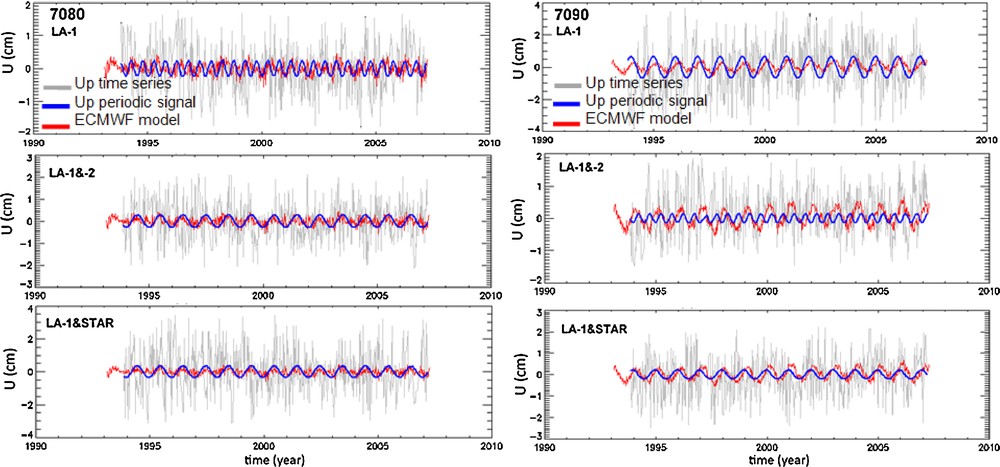
Comparison between seasonal signals of the Up components and atmospheric loading model (ECMWF) for 7090 and 7080 stations.
Comparaison entre les signaux saisonniers de la composante verticale Up et les charges atmosphériques (ECMWF), pour les stations 7090 et 7080.
Bruit affectant les signaux de la composante verticale (Up) de quelques stations SLR, suivant les différentes combinaisons. (Wh., Fl., ps) correspondent au bruit blanc, bruit de scintillation et signal périodique, respectivement.
| Station | Combination | Slope (cm/yr) |
Noise level (cm) |
Noise type |
| 7080 McDonald |
LA-1 | –0.6 | 0.3 | Wh. + weak Fl. |
| LA-1&-2 | –0.7 | 0.4 | Wh. + weak Fl. | |
| LA-1&STAR | –0.9 | 0.5 | Wh. | |
| 7090 Yarragadee |
LA-1 | –0.7 | 0.6 | Wh. + weak Fl. |
| LA-1&-2 | –0.6 | 0.3 | Wh. + weak Fl. Wh. | |
| LA-1&STAR | –0.9 | 0.4 | ||
| 7835 Grasse SLR |
LA-1 | –0.4 | 0.6 | Wh. + Fl. + ps. |
| LA-1&-2 | –0.5 | 0.6 | Wh. + Fl. + ps. | |
| LA-1&STAR | –0.7 | 0.7 | Wh. + ps. | |
| 7110 Monument Peak |
LA-1 | –0.5 | 0.3 | Wh. + Fl. |
| LA-1&-2 | –0.6 | 0.3 | Wh. + Fl. | |
| LA-1&STAR | –0.9 | 0.4 | Wh. |
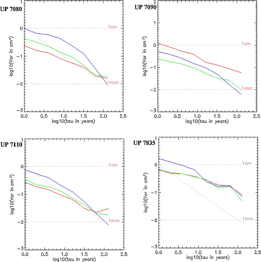
Allan variance graph of Up component updates of stations 7080, 7090, 7835 and 7110. The series corresponding to the satellites combinations are in red for LA-1, in green for LA-1&-2, and in blue for LA-1 & STAR.
Graphe de la variance d’Allan de la composante verticale Up des stations 7080, 7090, 7835 et 7110. Les séries temporelles correspondant aux combinaisons : LA-1 sont en rouge, LA-1&-2 sont en vert, LA-1&STAR sont en bleu.
5.2 Transformation parameters
Table 7 summarizes the statistics of the weekly series of Helmert transformation parameters (translation components and scale factor), between different combinations solutions and ITRF2005, and the daily series of pole motion parameters (pole coordinates and LOD).
Statistiques des paramètres de transformation (translations : TX, TY, TZ ; facteur d’échelle : D) et des paramètres du pôle (coordonnées résiduelles du pôle Xp, Yp et longueur du jour LOD) suivant les différentes combinaisons. Les valeurs de chaque paramètre représentent le minimum, le maximum, la moyenne et l’écart-type pondéré.
| Solution | TX (cm) |
TY (cm) |
TZ (cm) |
D (ppb) |
Xp (mas) |
Yp (mas) |
LOD (ms) |
|||||||
| LA-1 | –0.93 | 1.19 | –1.19 | 1.19 | –0.90 | 1.12 | –2.40 | 1.03 | –0.66 | 0.80 | –0.74 | 0.80 | –0.15 | 0.16 |
| 0.12 ± 0.49 | –0.27 ± 0.48 | 0.11 ± 0.46 | –0.66 ± 0.69 | 0.07 ± 0.26 | –0.01 ± 0.22 | 0.00 ± 0.03 | ||||||||
| LA-1&LA-2 | –0.92 | 1.00 | –0.85 | 1.00 | –0.79 | 0.78 | –1.87 | 0.76 | –0.50 | 0.61 | –0.52 | 0.61 | –0.11 | 0.11 |
| 0.03 ± 0.39 | –0.15 ± 0.35 | 0.00 ± 0.37 | –0.59 ± 0.56 | 0.05 ± 0.14 | –0.02 ± 0.13 | 0.00 ± 0.01 | ||||||||
| LA-1 &STAR | –1.04 | 1.65 | –1.22 | 1.65 | –1.22 | 1.17 | –2.18 | 1.80 | –0.65 | 0.92 | –0.72 | 0.92 | –0.16 | 0.17 |
| 0.30 ± 0.47 | –0.15 ± 0.46 | –0.04 ± 0.47 | –0.26 ± 0.75 | 0.14 ± 0.23 | 0.02 ± 0.20 | 0.00 ± 0.02 | ||||||||
| LA-1 &STARw | –0.85 | 1.68 | –1.39 | 1.68 | –1.08 | 1.51 | –5.10 | 1.09 | –0.64 | 0.83 | –0.65 | 0.83 | –0.15 | 0.15 |
| 0.39 ± 0.50 | –0.10 ± 0.50 | 0.23 ± 0.49 | –2.03 ± 0.78 | 0.10 ± 0.15 | 0.05 ± 0.15 | 0.00 ± 0.02 |
5.2.1 Geocenter variations
Among the weekly transformation parameters computed between the terrestrial reference frames (TRFs) and the ITRF2005, the translation parameters are of particularly importance. Indeed, they evidence the Geocenter variations. This is a topic of crucial importance in the Earth deformation theory as well as in the definition and maintenance of the ITRF.
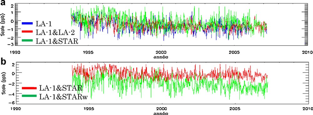
Fig. 4 illustrates the translation time series according to the different Laser measurement combinations of LAGEOS-1&-2 and Starlette satellites. It can be seen that the solution of the combination (LA-1&STAR) is slightly larger compared to the reference solution (LA-1&LA-2). Indeed, in the case of the LA-1&STAR combination, the dispersion is of about 2.7 cm for TX, 2.8 cm for TY and 2.4 cm for TZ, with average RMS of about ±5 mm. However, in the case of the reference solution, it is only of about 2 cm, 1.9 cm and 1.6 cm, for TX, TY and TZ, respectively, with mean RMS of about ±4 mm (Table 7).
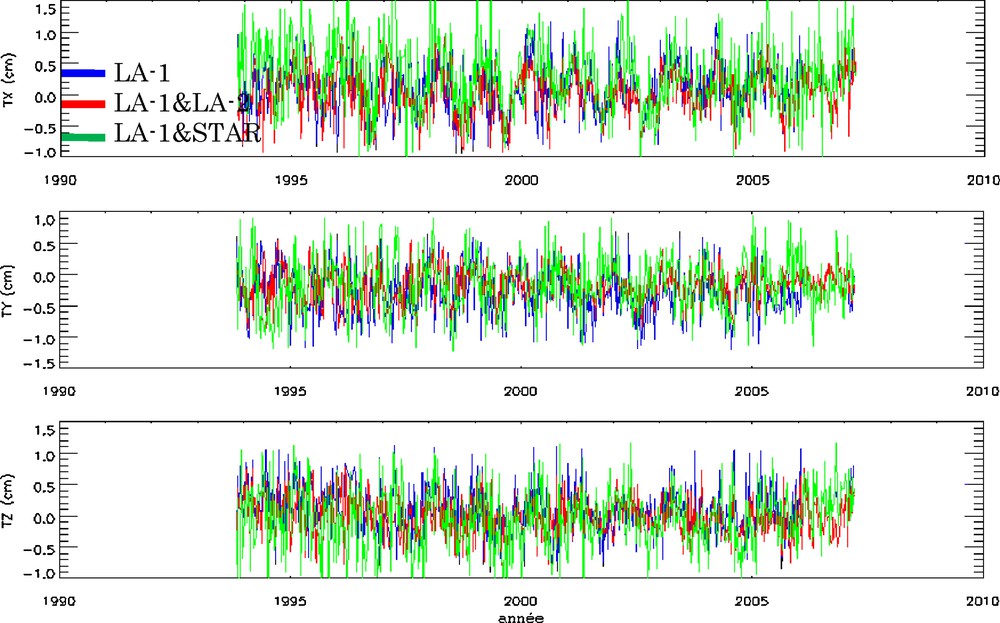
Time series of the Geocenter variations components (TX, TY, TZ).
Séries temporelles des composantes des variations du géocentre (TX, TY, TZ).
Fig. 5 shows a comparison between translation time series from (LA-1&STAR) and (LA-1&STARw) solutions. The latter is obtained by weighting the Starlette observations taking into account the corresponding standard deviations which are twice larger than those of LAGEOS performing the degree of freedom method (Coulot, 2005 for more details), in order to evaluate the effect of weighting on the results. It can be noted that the results are considerably equivalent for the parameters (TX and TY), and with a less degree, for the TZ component.
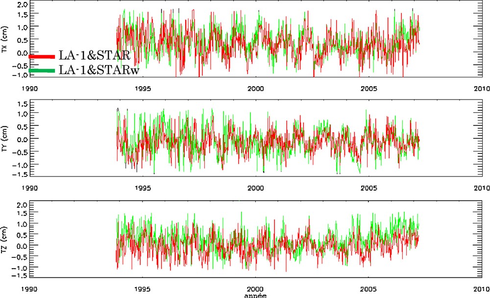
Comparison of the Geocenter variations components between LA-1&STAR and LA-1&STARw solutions.
Comparaison des composantes des variations du géocentre entre les solutions LA-1&STAR et LA-1&STARw.
The Geocenter variations are mainly due to the redistribution of masses in atmosphere, in oceans and also in hydrological reservoirs. In general, they present two principal periodic components: annual and semi-annual terms. Table 8 displays the values of amplitudes and phases of annual and semi-annual terms of our solutions, ILRS solution (Collilieux et al., 2009), and two geophysical models of Chen et al. (1999) and Dong et al. (1997), computed taking into account atmospheric pressure data, ocean tides and surface water data. The comparison between LA-1&STAR results and those of the other authors revealed agreements at millimeter level for the amplitudes. Better agreements for annual and semi-annual terms, of LA-1&STARw compared to ILRS solution and both geophysical models in the TX and TY components.
Comparaison entre les termes saisonniers des composantes du Géocentre (TX, TY, TZ) et des variations du facteur d’échelle (D) des différentes combinaisons avec les estimations de l’ILRS (Collilieux et al., 2009) et les modèles géophysiques de Chen et al. (1999) et Dong et al. (1997). A etφ sont, respectivement, l’amplitude en mm et la phase en degrés.
| Parameter | Combinations solutions | ILRS | Chen et al. (1999) | Dong et al. (1997) | |||
| LA-1&STARw | LA-1&-2 | LA-1&STAR | LA- | ||||
| TX A 1 yr | 2.3 ± 0.3 | 2.4 ± 0.3 | 3.3 ± 0.4 | 2.4 ± 0.4 | 2.7 ± 0.3 | 2,4 | 4,2 |
| TX φ 1 yr | 279.5 ± 16.7 | 280.4 ± 13.7 | 300.5 ± 11.9 | 296.4 ± 15.7 | 45 ± 6 | 244 | 224 |
| TX A ½ yr | 0.7 ± 0.2 | 0.8 ± 0.3 | – | 0,7 | 0,8 | ||
| TX φ ½ yr | 277.6 ± 42.9 | 96.2 ± 50.6 | 1 | 210 | |||
| TY A 1 yr | 1.5 ± 0.2 | 1.1 ± 0.3 | 2.0 ± 0.2 | 3.1 ± 0.6 | 3.8 ± 0.2 | 2,0 | 3,2 |
| TY φ 1 yr | 88.9 ± 25.0 | 65.1 ± 22.2 | 0.1 ± 20.4 | 51.9 ± 10.9 | 327 ± 4 | 270 | 339 |
| TY A ½ yr | 0.9 ± 0.4 | – | 0,9 | 0,4 | |||
| TY φ ½ yr | 337.7 ± 43.8 | 41 | 41 | ||||
| TZ A 1 yr | 1.3 ± 0.5 | 1.3 ± 0.3 | 2.3 ± 0.4 | 2.2 ± 0.3 | 3.6 ± 0.4 | 4,1 | 3,5 |
| TZ φ 1 yr | 322.9 ± 23.3 | 332.1 ± 17.6 | 290.9 ± 16.8 | 261.4 ± 21.0 | 4 ± 7 | 228 | 235 |
| TZ A ½ yr | – | 0,5 | 1,1 | ||||
| TZ φ ½ yr | 58 | 133 | |||||
| D A 1 yr | 0.7 ± 0.3 | 0.6 ± 0.2 | 1.0 ± 0.3 | 2.0 ± 0.5 | 1.7 ± 0.2 | – | – |
| D φ 1 yr | 201.7 ± 35.8 | 96.1 ± 35.8 | 189.4 ± 29.6 | 29.0 ± 17.6 | 144 ± 8 | ||
| D A ½ yr | 0.7 ± 0.3 | 0.9 ± 0.3 | 0.7 ± 0.2 | – | – | ||
| D φ ½ yr | 20.7 ± 33.2 | 257.9 ± 32.7 | 3 ± 17 |
For phases, the agreements are less convincing. This is probably due to the choice of reference frame and physical models used in the computations (Coulot and Berio, 2006). The spectral behavior of time series of Geocenter motion, described by the method of the Allan variance, is shown in Fig. 6a. After removing the trend (estimated by linear regression) and the periodic components (annual and semi-annual terms), we applied the Allan variance on the resulting Geocenter motion time series. The dominant noise type in these series is white noise. However, the noise affecting the three Geocenter components of LA-1&STAR solution is slightly important, being about 2 mm. The solution (LA-1&LA-2) remains the least disturbed with a noise level of about 1 mm. On the other hand, Table 9 and Fig. 6b show that the weighting of Starlette measurements affected only the TZ component where the type of noise is a flicker noise, with the same order of 2 mm.
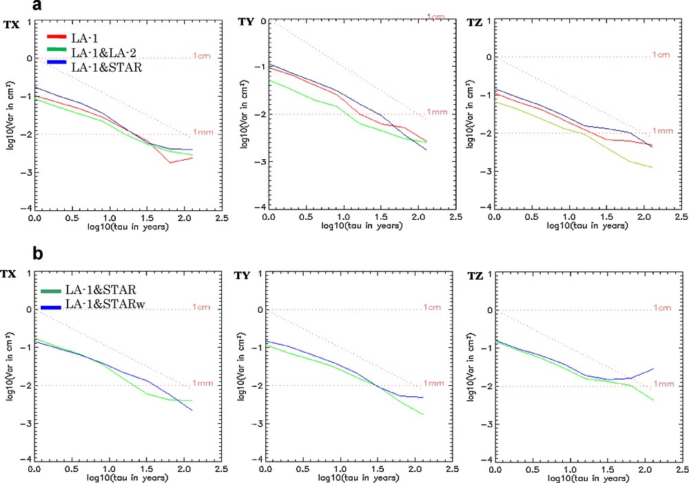
Allan variance of Geocenter variation components according to: a: all combination solutions (LA-1, LA-1&LA-2 and LA-1&STAR); b: solutions (LA-1&STAR and LA-1&STARw).
Variance d’Allan des composantes du Géocentre suivant : a : les solutions (LA-1, LA-1&LA-2 et LA-1&STAR) ; b : les solutions (LA-1&STAR et LA-1&STARw).
Bruit des séries temporelles des paramètres de transformation et du facteur d’échelle. La pente du graphe log-log de la variance d’Allan désigne le type du bruit et NL est le niveau de bruit.
| TX (cm) |
TY (cm) |
TZ (cm) |
D (ppb) |
|||||
| Solution | Slope | NL | Slope | NL | Slope | NL | Slope | NL |
| LA-1 | –0.9 | 0.16 ± 0.01 | –0.8 | 0.16 ± 0.01 | –0.7 | 0.16 ± 0.01 | –0.6 | 0.28 ± 0.02 |
| LA-1&LA-2 | –0.7 | 0.14 ± 0.01 | –0.7 | 0.12 ± 0.004 | –0.9 | 0.12 ± 0.01 | –0.6 | 0.22 ± 0.01 |
| LA-1 &STAR | –0.7 | 0.19 ± 0.02 | –0.8 | 0.17 ± 0.01 | –0.7 | 0.19 ± 0.01 | –0.8 | 0.32 ± 0.04 |
| LA-1 &STARw | –0.8 | 0.19 ± 0.01 | –0.8 | 0.19 ± 0.01 | –0.5 | 0.22 ± 0.01 | –0.8 | 0.46 ± 0.08 |
5.2.2 Scale factor variations
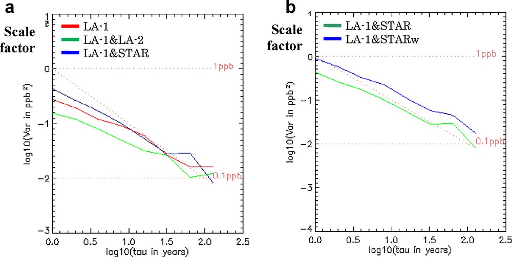
Scale factor variations of the reference frame are affected by errors of the stations’ vertical component determination (Coulot, 2005). Thus, the range biases and errors on the radial components due to residual orbital errors, which limit the accuracy of the vertical components, affect the scale factor variations. On the other hand, the network effect (Collilieux and Altamimi, 2008) is another factor that may also affect the scale factor. Fig. 7 shows the time series of the scale factor variations, corresponding to different combinations.
Time series of scale factor according to: a: different combination solutions (LA-1, LA-1&LA-2 et LA-1&STAR); b: solutions from un-weighted and weighted Starlette measurements (LA-1&STAR and LA-1&STARw).
Séries temporelles du facteur d’échelle suivant : a : les solutions des différentes combinaisons (LA-1, LA-1&LA-2 et LA-1&STAR) ; b : les solutions (LA-1&STAR et LA-1&STARw).
From Table 7, the dispersion of the (LA-1&STAR) series is of the order of 4.0 ppb with an RMS of ±0.56 ppb (or 24 ± 5 mm). In the case of LAGEOS solutions, it is about of 2.7 ppb with RMS of ±0.75 ppb (or 16 ± 3 mm). This shows that Starlette measurements are noisier than LAGEOS ones. Fig. 7b and Table 7 show a shift in magnitude of about 1.8 ppb (or 11 mm) between both time series of LA-1&STAR combinations (weighted and un-weighted measurements of Starlette).
Table 8 provides the values of annual signals and/or semi-annual (amplitudes and phases) of the scale factor. LA-1&STAR solution contains both periodic components with an amplitude of about 0.17 ppb/yr and 0.15 ppb/06 months (1 mm/yr and 0.9 mm/06 months; slightly higher values compared to those of LAGEOS solutions but with the same RMS). However, the annual amplitude of the LA-1&STARw solution, which is approximately twice larger than LA-1&STAR one, agrees well with ILRS amplitude.
Fig. 8 shows the graph of the Allan variance of time series of the scale factor. It can be seen that the dominant noise for combinations using measurements of Starlette is a white noise of about 2 to 3 mm level. For LAGEOS solutions, one notices, in addition to white noise, the presence of flicker noise with a level of 1 to 2 mm (Table 9).
Allan variance of Scale factor according to: a: all combination solutions (LA-1, LA-1&LA-2 and LA-1&STAR); b: solutions (LA-1&STAR and LA-1&STARw).
Variance d’Allan des séries temporelles du facteur d’échelle suivant : a : les solutions (LA-1, LA-1&-2 et LA-1&STAR) ; b : les solutions (LA-1&STAR et LA-1&STARw).
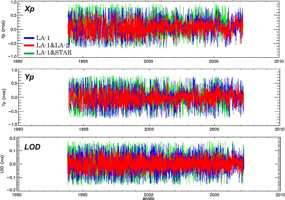
5.3 EOP parameters residuals
Fig. 9 presents the time series residuals of the pole coordinates (Xp, Yp), and of the LOD. These times series were processed, for different solutions, with respect to the standard solution EOPC04 of IERS, and expressed according to a coherent reference frame with ITRF2005. From Table 2, the standard deviations of the (LA-1&-2) solution are, respectively, of about 0.14 mas (∼4 mm), and 0.01 ms (∼5 mm) for the pole coordinates and time.
Time series of pole motion parameters (Xp, Yp, LOD).
Séries temporelles des paramètres du pôle (Xp, Yp et LOD).
According to the LA-1&STAR solution, the RMS are slightly large, in the range of 0.20 to 0.23 mas (or, 6–7 mm) for pole coordinates, and 0.02 ms (or 10 mm) for LOD. In addition, the estimation of pole parameters is satisfactory for the SLR technique and the obtained values are coherent with published values of IERS, which are at a level of 200–300 μas (Gambis, 2004).
Fig. 10 shows an agreement between both time series of the LA1&STAR solutions, in the case of weighted and un-weighted Starlette observations. In fact, in terms of RMS, the two series are at a level of 5 to 6 mm for pole coordinates and of about 10 mm for LOD; Table 2. The EOP solutions obtained by SLR technique appear to be inconsistent with EOPC04 at level of 5 to 10 mm (∼200 to 300 μas) (Gambis, 2004).
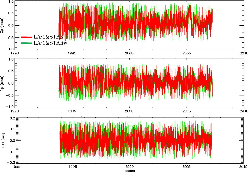
Time series of pole motion parameters (Xp, Yp, LOD) according to LA-1&STAR and LA-1&STARw solutions.
Séries temporelles des paramètres du pôle (Xp, Yp, UT et LOD) suivant les solutions LA-1&STAR et LA-1&STARw.
Table 10 depicts the results of frequency analysis of pole parameters series, using FAMOUS software. The periodic signals are decomposed, with respect to three periods: inter-annual, annual and short periods (from few days to few months < 100 days). The choice of this decomposition is based on the periods of the geophysical phenomena causing the variations in the pole motion. These phenomena are mainly due to the redistribution of masses in the Earth, oceans and atmosphere (Frède, 1999).
Signaux périodiques des paramètres du pôle (Xp, Yp et LOD).
| Parameter | Period | LA-1 | LA-1&LA-2 | LA-1&STAR | LA-1&STARw |
| Xp (μas) | Inter-annual | 56.3 | 30.1–40.8 | 36.1–48.3 | 33.2–36.6 |
| Annual | – | 31.9 | 46.7 | 32.6a | |
| Short period | 30.4–34.1 | 23.6–28.5 | 34.5–41.3 | 31.7 | |
| Yp (μas) | Inter-annual | 46.0 | – | 39.0 | 33.0 |
| Annual | 39.7 | 35.0 | 72.9 | 74.4 | |
| Short period | 31.4–34.0 | 10.6–22.2 | 31.3–36.1 | 28.1–37.2 | |
| LOD (μs) | Inter-annual | 6.4 | – | 6.5 | – |
| Annual | 5.9 | 6.0 | – | 7.2 | |
| Short period | 5.4–6.0 | 3.5–4.1 | 6.1–13.8 | 5.8–13.7 |
a Corresponds to semi-annual term.
The results of different combinations are very close, because the maximum amplitudes of different signals of polar motion do not exceed 74 μas (or 2.2 mm). As can be observed, the residual effects of geophysical phenomena, mentioned above, on the polar motion, are weak and of about few millimeters. For LOD, the variations are induced by the friction of the winds and ocean currents on the solid Earth surface (Frède, 1999). Similarly, variations of this parameter can be decomposed into three terms. The estimated amplitudes of these terms range from about 4 to 6 μs (approximately 2–3 mm) for LAGEOS combinations and are around 7 to 14 μs (or 4–7 mm) for Starlette and LAGEOS-1 combinations. Generally, these values remain very small because they describe the residual signals of the geophysical phenomena.
According to Table 11, all the combinations are characterised by a flicker noise, with levels of about 3 mm and 4 mm in polar motion, 9.5 mm and 14.5 mm in LOD, for LA-1&LA-2 and LA-1&Star, respectively.
Bruit des paramètres du pôle. La pente du graphe log-log de la variance d’Allan désigne le type du bruit et NL est le niveau de bruit.
| Solution | Xp (μas) | Yp (μas) | LOD (μs) | |||
| Slope | NL | Slope | NL | Slope | NL | |
| LA-1 | –0.4 | 140 ± 2 | –0.5 | 130 ± 3 | –0.7 | 26 ± 0.3 |
| LA-1&LA-2 | –0.4 | 110 ± 1 | –0.4 | 90 ± 1 | –0.7 | 19 ± 0.1 |
| LA-1&STAR | –0.5 | 140 ± 3 | –0.4 | 0.14 ± 2 | –0.7 | 29 ± 0.2 |
| LA-1 &STARw | –0.5 | 140 ± 3 | –0.4 | 0.13 ± 2 | –0.6 | 27 ± 0.1 |
6 Conclusion
In this study, we analysed the different SLR data combinations, namely LA-1, LA-1&LA-2 and LA-1&STAR, in order to study the contribution of Starlette laser measurements in the determination of the geodetic products. An average arc RMS of about 1–2 cm has been obtained for LAGEOS-1&-2 and Starlette satellites. The stations positioning accuracy according to the local geodetic coordinates (Northing, Easting, Up) is at centimeter level. Small but significant degradation of RMS of about 3 to 5 mm is observed when adding Starlette data, but also a better capability to determine the annual and semi-annual variations of the UP component and, as a result, very probably a capability to determine the station coordinates if no LAGEOS data were available. The RMS obtained on Geocenter variation components are the same for different combinations of about 4 to 5 mm, and are at level of 0.14 to 0.20 mas (∼4–6 mm) on pole coordinates, and 0.01 to 0.02 ms (∼5–10 mm) on LOD, for EOP, which are in good agreement with the values of IERS.
The proposed analysis methodology was based on: frequency analysis; and noise estimation of the time series of the parameters of interest. The combinations of Starlette and LAGEOS-1 data give better results for seasonal signals, which are in good agreements with ILRS terms and geophysical models in the TX and TY components. The type of dominating noise is the white noise, with a level of about 2 mm. The EOP periodic signal is decomposed into inter-annual, annual and short period terms. The flicker noise is the characterizing noise of the EOP time series with a level of about 4 and 15 mm in pole coordinates and LOD, respectively, for the LA-1&STAR solutions. On the basis of these results, it is interesting to perform a more global analysis of different geodetic LEO satellites data in the estimation and interpretation of the geodetic SLR products.
Acknowledgments
Special thanks are given to the GMC team (P. Exertier, P. Berio, D. Feraudy and D. Coulot, etc.) from Observatoire de la Côte d’Azur (OCA), Grasse, France, for their precious technical aid and scientific assistance to achieve this work. The author also thanks S. Kahlouche and B. Ghezali from CTS (Algeria).
1 Web site of the International Laser Ranging Service (ILRS): http//ilrs.gsfc.nasa.gov/.