

1 Introduction
In 1988, Jan Veizer proposed that the time evolution of the surficial envelopes of the Earth was driven by a hierarchy of processes (Veizer, 1988). At the geological timescale (106 to 109 years), the dominant process controlling the long term changes in the oceanic and atmospheric chemistry, and hence climate, was proposed to be tectonics. In Veizer's view, biological processes are piggybacking on tectonics, and are not driving the long term evolution of the Earth surface. They only adapt to the tectonic forcing. The cross correlation observed between the various isotopic signals measured in Phanerozoic sedimentary carbonates (87Sr/86Sr, δ13C, δ18O) supports this hypothesis (Veizer et al., 1999).
This theory assuming the predominant role of tectonics on the chemical evolution of the Earth surface is challenged by ideas supporting a predominant impact of life on Earth, at least during time periods marked by critical steps in the evolution of life. A well-known example is the accumulation of oxygen in the atmosphere in response to the appearance of the oxygenic photosynthesis. Apparently, subsequent to the oxygenation of the surficial envelopes, atmospheric methane levels decreased drastically, leading to the first severe glaciation at the Earth surface in the Early Proterozoic (Catling and Claire, 2005; Kasting and Ono, 2006; Kopp et al., 2005; Kump, 2008). The invasion of the continental surfaces by land plants during the Devonian is also supposed to have strongly modified the weathering regimes at the Earth surface, and hence the atmospheric CO2 level and the global climate (Berner, 2004). Strikingly, the evolution of life has been proposed also to trigger the onset of cold climatic conditions, here the Permo-Carboniferous glacial event. Terrestrialization may have even impacted the subduction rates, as suggested by non equilibrium thermodynamic considerations (Dyke et al., 2011). In addition, the development of the mycorrhizosphere around plant roots is also thought to have boosted the weathering rates (Taylor et al., 2012). A last example often cited is the evolution of the calcareous nanoplankton which has strongly modified either the chemical gradient in the oceans and possibly the global climate with the emission of dimethyl sulfide into the atmosphere (Westbroeck, 1992).
Is life a climate driver on geological scales, or is tectonics the only forcing function? It is rather difficult to discriminate between the two scenarios. Indeed, for two of the above examples, tectonics may be invoked as the ultimate cause of change, even if life evolution is involved. In the case of the Precambrian oxygen rise, production of oxygen is not sufficient for it to accumulate in the surficial envelopes. It is a matter of relative budget: either the source of O2 must have increased around 2.3 Gyr, or the sink must have declined (Catling and Claire, 2005; Veizer, 1988). For instance, it may be argued that the presence of large continents is required for the nutrients to be supplied by weathering for the biosphere, so that it can support a large oxygen production (Goddéris and Veizer, 2000). Large continents are also required to provide large continental shelves that will be colonized by oxygen producers. So the oxygenation may depend on accretion of new continents around the Archean/Proterozoic boundary that led to transition from the early “mantle-buffered” to the “river-buffered” oceans (Veizer and Mackenzie, 2004), that is, from the scenario where, due to declining geothermal head flux, the early highly reducing fluxes from the ubiquitous submarine hydrothermal circulation cells and volcanism were superposed by more oxidized subaerial volcanism (Kump and Barley, 2007).
Similarly, the rise in nanoplankton producers at the end of the Triassic may have been related in part to changes in carbon cycle and climate linked to the northward drift of Pangea (Goddéris et al., 2008). This latter drift is thought to have enhanced continental rock weathering and associated CO2 consumption, promoting carbonate production in seawater under less acidic conditions. At the same time, coral reefs might have been boosted by this CO2 decrease (Kiessling, 2010). Biological and tectonic forces are also tightly intertwined when considering the role of mountain uplift on the carbon cycle and climate evolution. The proposition that mountain uplift, due to increased erosion, drives CO2 consumption (Raymo and Ruddiman, 1992) and initiates glaciation may be incomplete from the carbon budget perspective because Goddéris and François (1995) and Kump and Arthur (1997) demonstrated that mountain ranges do not increase the overall CO2 consumption by weathering. Instead they may contribute to CO2 drawdown via enhanced regional weatherability that measures susceptibility of a given continental surface to prescribed climatic conditions. Moreover, in the peculiar case of the Himalayan uplift, the high sedimentation rates induced by intense erosion in fact leads to an efficient burial of organic carbon that is mostly of terrestrial origin (France-Lanord and Derry, 1997; Galy et al., 2007). This is another illustration of the tight coupling that may exists between tectonic and biological processes.
2 Aims and method
In this contribution, we aim at isolating the tectonic control on the geological evolution of the carbon cycle and climate. The two main “geological” forcings are tested: the continental drift and the fluctuations in the solid Earth degassing. Although mountain ranges are considered in this study as climatic barriers, we do not account explicitly for their possible geochemical effects such as increased erosion that is potentially promoting organic carbon burial and local weatherability. Nevertheless, physical erosion is accounted for in a simple way (see below).
We use the climate-carbon model GEOCLIM to reconstruct the temporal evolution of the Phanerozoic CO2 and climate in response to continental drift and to variability in the degassing rate of the solid Earth (Donnadieu et al., 2006, 2009). GEOCLIM couples a 3D climate model (the FOAM GCM; Jacob, 1997) to a model of the global biogeochemical cycles (COMBINE; Goddéris and Joachimski, 2004). For 21 continental configurations spanning the entire Phanerozoic, we calculate the atmospheric CO2 assuming that the paleothermostat equation is verified (Walker et al., 1981):
| (1) |
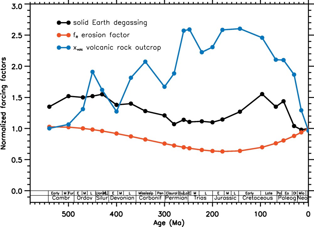
Three forcing function of the reference simulation. Additional input includes continental configuration and increasing solar constant with time. All functions are normalized to their present day value and taken directly from Berner (2004).
Les trois fonctions de forçage de la simulation de référence, outre la configuration continentale et la croissance de la constante solaire au cours du temps. Toutes les fonctions sont normalisées à leur valeur actuelle et sont tirées de Berner (2004).
The specificity of GEOCLIM, compared to other geological climate-carbon models, lies in the method used to calculate Fsilw (Fig. 2). Different from previous adimensional models (such as GEOCARB, Berner, 2004), GEOCLIM resolves the continental runoff and mean annual air temperature above the continents with a spatial resolution of 7.5° long. × 4.5° lat. (Donnadieu et al., 2006). GEOCLIM is also the only numerical model of its type to allow a process-based calculation of the water cycle. Continental runoff, a key parameter of the weathering reactions, is explicitly calculated by the 3D climate model as the difference between rainfall and evapo-transpiration above each continental grid cell. This allows GEOCLIM to capture accurately the impact of the continental configuration on the runoff pattern. In other models, global runoff is estimated through simple phenomenological laws calibrated on the present continental configuration. The impact of continental drift on runoff is accounted for by offline GCM simulations performed at 1 PAL CO2, inducing inconsistencies between the calculated state of the carbon cycle and of the climate at each timestep (GEOCARB model; Berner, 2004).
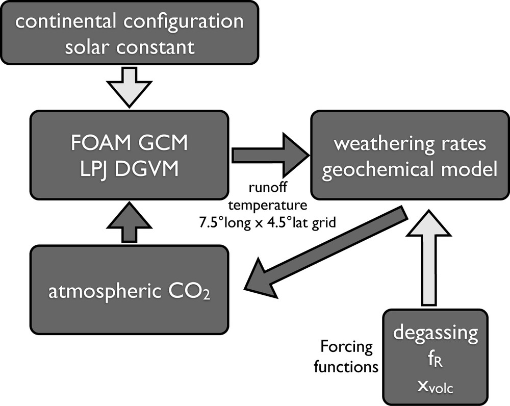
Description of the GEOCLIM model. For each continental configuration, the climate output of the coupled FOAM climate model and of LPJ dynamic global vegetation model are used to calculate the continental weathering rates, and hence the atmospheric CO2 level for which consumption by weathering precisely balances the solid Earth outgassing. The three additional forcing function (variable degassing, fR and xvolc) are only used in the reference simulation.
Description du modèle GEOCLIM. Pour chaque configuration continentale, les sorties climatiques du modèle de climat FOAM couplé au modèle dynamique de végétation globale LPJ sont utilisées pour calculer les taux d’altération continentale, et donc la pression de CO2 atmosphérique pour laquelle la consommation de CO2 par altération compense le taux de dégazage volcanique. Les trois fonctions de forçage supplémentaires (dégazage variable, fR and xvolc) ne sont utilisées que pour la simulation de référence.
GEOCLIM also includes a dynamic calculation of the distribution of the continental vegetation, via full coupling of the FOAM 3D climate model with the Lund-Postdam-Jena global dynamic vegetation model (Donnadieu et al., 2009). Prior to Devonian, continents are assumed to have been rocky deserts. We are aware that this may be an oversimplification given that early land plants evolved in the Late Ordovician. However, the physical parameters and the spatial extent of this early vegetation are too poorly known to allow a realistic representation in a global numerical model. For Devonian and post-Devonian timeslices, the LPJ model is used with present day plant functional types.
By incorporating a dynamic vegetation in our modeling, we implicitly include an impact of life on the temporal evolution of the global climate. However, we only model the biophysical impact of the vegetation on climate, i.e. changes in albedo and in the roughness of the continental surfaces. The role played by vegetation on the global water cycle is accounted for through modifications of the evaporation capability as a function of the vegetation type. As developed in Donnadieu et al. (2009) and Le Hir et al. (2011), when climate changes in response to continental drift, the distribution of the continental vegetation changes, feedbacking on the climate and water cycle, and hence on the weathering processes. However, in order to limit the biological impact on the long term carbon cycle evolution, we do not account for a direct impact of the biosphere on the weathering rates through time at this stage (enhancement of weathering by root respiration, mechanical effect of roots, release of organic acids).
The Fsilw term is calculated for each continental grid cell through a parametric relationship linking mean annual runoff and air temperature to CO2 consumption by weathering (Dessert et al., 2003; Donnadieu et al., 2006; Oliva et al., 2003). Those phenomenological rate laws were calibrated over one hundred small monolithological watersheds, through the measurements of their present day CO2 consumption by weathering and its correlation with local runoff and mean annual air temperature. The compiled watersheds span a large variety of climate and vegetation cover. By using these laws even for pre-Devonian times, we implicitly neglect any direct impact of the land plant evolution and root systems on the weathering rates, which makes sense since we aim at isolating as far as possible the tectonic forcing (continental drift) of the climatic evolution of the Earth.
Several modulating factors of weathering rates have been introduced in GEOCLIM if compared to previously published versions. We account for the change in the relative outcrop of young basaltic rocks versus old igneous rocks. Mathematically speaking, the 87Sr/86Sr isotopic ratio of sedimentary carbonates is used to estimate xvolc, i.e. the ratio of young basaltic rock outcrops versus total continental area (see Berner, 2004 for details; Fig. 1). We also account for a fluctuating role of physical erosion (fR factor, also taken from the GEOCARB model of Berner, 2004) (Fig. 1). Eq. (1) can thus be rewritten as follows:
| (2) |
3 Results and discussion
3.1 Atmospheric CO2 levels
Two simulations have been performed. First, the reference simulation assumes a variable solid Earth degassing rate, a variable erosion fR and a variable young volcanic rocks ratio xvolc. Second, the TEC simulation has been run with all these three parameters set at their present day value, allowing us to clearly depict the only effect of continental configuration on atmospheric CO2.
Regarding the calculated atmospheric CO2 content, the salient features of both simulations can be summarized as follows (Fig. 3):
- • the Early Paleozoic period is characterized by a major atmospheric CO2 decrease;
- • the Triassic and the Cambrian are marked by very high CO2 levels;
- • since the Middle Cretaceous (around 100 Ma in the reference run, slightly earlier in the TEC run which displays overall lower CO2 levels), the calculated CO2 level is rapidly declining from 6 PAL (reference run) down to the present day value.
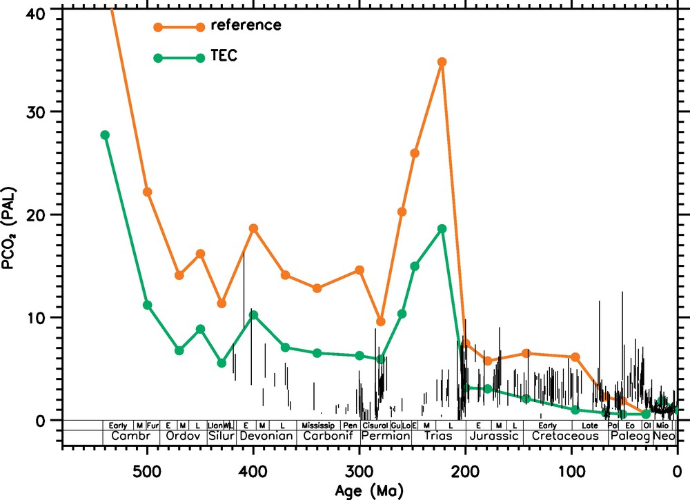
Calculated evolution of the atmospheric CO2 pressure over time, using the GEOCLIM model for the reference and the TEC (where the only forcings are the continental configuration and the solar constant) simulations (1 PAL = 280 ppmv). Also shown (vertical black lines) is the latest update of the CO2 proxy database (Breecker et al., 2010; Royer et al., 2007).
Évolution calculée par le modèle GEOCLIM de la pression de CO2 atmosphérique, pour les simulations de référence et TEC (pour laquelles les deux seuls forçages sont la configuration continentale et la constante solaire) (1 PAL = 280 ppmv). La dernière version de la base de données du niveau de CO2 est également figurée (barres verticales noires) (Breecker et al., 2010 ; Royer et al., 2007).
In detail, the high Paleozoic values are mainly forced by the low solar constant. Atmospheric CO2 is forced to rise to compensate for the low insolation, so that silicate weathering is sustained and the paleothermostat equation is verified (Eq. (1) and (2)). However, a major drop in CO2 levels is calculated from the Mid-Ordovician to the Llandovery. The cause of this drop is of tectonic origin. In detail, this is the northward drift of the three main continental blocks (Laurentia, Siberia and Baltica) that maximizes the CO2 consumption by silicate weathering, forcing atmospheric CO2 to decrease and climate to get colder (Nardin et al., 2011).
The second period when continental configuration plays a dominant control on the global carbon cycle is the Triassic. Very high CO2 levels are calculated from the Lopingian period up to the Carnian stage of the Triassic, from about 5500 up to 9800 ppmv. These high CO2 levels are directly related to the shaping of the Pangea supercontinent at the same time. Because of increasing continentality, runoff is maintained at low levels, and the climate system warms so that temperature and runoff are eventually high enough for silicate weathering to compensate for the solid Earth degassing (Donnadieu et al., 2006; Gibbs et al., 1999; Goddéris et al., 2008). These high levels are sustained as long as the supercontinental configuration inhibits runoff. In the latest stage of the Triassic (Rhetian), the northward drift of Pangea increases the continental surface located in the intertropical convergence zone, thus promoting silicate weathering and forcing CO2 to decrease (Goddéris et al., 2008). After the Latest Triassic, persisting low CO2 levels are maintained by the fragmentation of the Pangea, promoting runoff, and hence silicate weathering.
The latest marked event is the decrease in atmospheric CO2 over the last 100 million years (150 million years in the TEC run). Although it may appear moderate compared to older CO2 excursions, its climatic impact is important given that climate sensitivity increases at low CO2 levels because of the logarithmic dependence of the climate on the CO2 level. This continental weatherability increase and subsequent CO2 decrease are the consequences of the ongoing breakup of the Pangea. Following the opening of the South Atlantic after the Berriasian, the northern part of Africa and South America stays in the convergence zone during this period, allowing an intense CO2 consumption by weathering (Fig. 4).
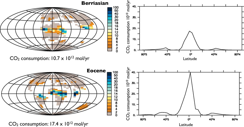
Calculated CO2 consumption by silicate weathering for the Berrisian stage of the Cretaceous to the Eocene. Calculations were performed under 1 PAL (280 ppmv) of atmospheric CO2. Shown is the spatial and latitudinal distribution of the flux, on 1010 mol of CO2/yr. The number is the total CO2 consumption in 1012 mol/yr, illustrating the weatherability increase from the Cretaceous towards the Cenozoic.
Consommation de CO2 par l’altération des silicates pour l’étage Berriasien du Crétacé et pour l’Éocène. Les calculs ont été effectués pour une pression de 280 ppmv de CO2 atmosphérique (1 PAL). La distribution spatiale et la répartition en latitude du flux sont montrées en 1010 mol CO2/an. Le nombre isolé donne la consommation totale de CO2 en 1012 mol/an, illustrant l’augmentation de l’altérabilité du Crétacé au Cénozoïque.
3.2 Temperature trends
A striking feature of the reference simulation is the prediction of the lowest global temperature in the Late Cenozoic (Fig. 5). All other periods of the Phanerozoic are predicted to be warmer by at least 5 °C. The same conclusion holds for the continental temperature with the Oligocene, Miocene and present day temperatures about 8 °C below the Paleozoic-Mesozoic mean value. The warmest continents are predicted in the Middle Triassic, with a mean annual temperature in excess of 25 °C.
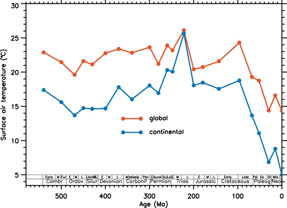
Calculated time evolution of the global mean air temperature and continental mean air temperature, for the reference simulation.
Évolution temporelle calculée de la température moyenne de l’air globale et continentale dans la simulation de référence.
Comparing these temperature outputs to available data (from δ18O measured on sedimentary apatite or carbonate) might not be fully relevant. Indeed, our model only calculates the multi-million year steady-state CO2, corresponding to the climate required for silicate weathering to balance the volcanic outgassing. Many other possible forcing functions are missing, such as the organic carbon burial and its impact on the global carbon cycle.
However, trends can be identified. We performed a frequency analysis of the temperature calculated for the tropical surface ocean (30°N–30°S) over the whole Phanerozoic in the standard simulation. The spectrum shows the dominance of the 115 Myr period, close to the 132 Myr period calculated from the Phanerozoic δ18O database for the tropical seawater (Prokoph et al., 2008) and to the 135 Myr calculated by Veizer et al. (2000) from an older version of the δ18O database (Fig. 6). This periodicity, observed also in the compilation of Phanerozoic glacial deposits (Frakes et al., 1992; Veizer et al., 2000) was never explained before. Our results suggest that it may be linked to the continental drift and its control on the weathering fluxes. Indeed, if we assume a constant degassing rate, a constant xvolc and fR (both fixed at their present day value), the only remaining forcings are the linear rise in the solar constant and the continental drift (TEC simulation). The sea surface tropical temperature calculated by GEOCLIM still displays a strong periodicity signal at 115 Ma (Fig. 6). Consequently, the continental drift over the Phanerozoic, by successively promoting or inhibiting continental weathering, strongly contributes to the observed periodicity of the tropical temperature signal.
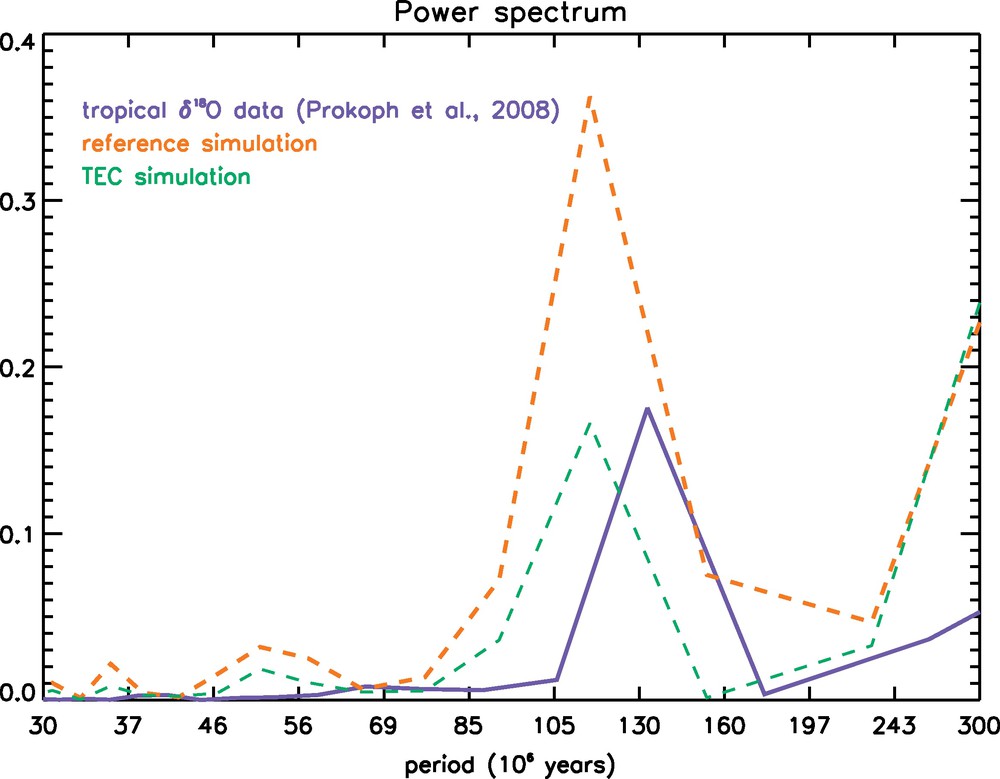
Power spectrum of the Fourier analysis of the averaged tropical sea surface temperature (30°S–30°N) calculated in the reference and TEC simulations. Data are from Prokoph et al. (2008) and based on carbonate δ18O.
Spectre de puissance résultant de l’analyse de Fourier de la température moyenne des eaux de surface tropicales (30°S–30°N), calculée dans les simulations de référence et TEC. Les données de δ18O acquises sur carbonates sédimentaires proviennent de Prokoph et al. (2008).
4 Temperature and CO2 changes over time
Is it possible to estimate the absolute CO2 level in the past? Many studies have dealt with this question from a proxy point of view. Absolute CO2 levels have been reconstructed over the last 450 million years from stomatal index of fossil leaves, from δ13C of pedogenic carbonates, from the biospheric carbon isotopic fractionation in the ocean among other methods (Royer et al., 2001). While those proxies can provide very different results (Goddéris et al., 2008), publications of the last years tend to lower the estimates of CO2. For instance, despite the existence of studies showing high levels of CO2 in the Middle Miocene (Kürschner et al., 2008), there is a real fascination for studies suggesting very low levels during this warm interval (below the pre-industrial value, Pagani et al., 2005). Recently, Breecker et al. (2010) have drastically reduce the Paleozoic and Mesozoic CO2 values through a recalibration of the pedogenic carbonate method. We are now left with level as low as 1000 ppmv in the Devonian, or below 1000 ppmv in the Early Triassic (Fig. 3).
Conversely, seawater temperatures calculated from proxies for the deep time tends to increase in the most recently published dataset. Ten years ago, the δ18O carbonate data predict very high temperatures in the seawater, particularly for the Paleozoic, because they display a general decreasing trend as we go back into the past (Veizer et al., 1999). However, δ18O ratio measured on well preserved apatite (mainly conodonts for the Paleozoic, then fish teeth for more recent periods) suggested lower temperatures than coeval carbonate samples, casting doubt on the reliability of the carbonate data. However, a recent recalibration of the apatite paleothermometer by Pucéat et al. (2010) warms up apatite-based temperatures by at least 4 °C, so that they display now high temperatures, close to the temperatures inferred from carbonate data. For instance, tropical sea surface temperatures reconstructed from conodont apatite now reaches 37 to 38 °C in the Devonian when the new paleothermometer is used (Fig. 7), while it was never exceeding 32 °C (Joachimski et al., 2009) with the former paleothermometer (Kolodny et al., 1983). Such high temperatures cannot be reached with only 1000 ppmv of CO2, given that the solar constant is reduced by 3%. For instance, GEOCLIM calculates a mean tropical SST of only 30 °C with more than 4200 ppmv of CO2 (15 PAL). Regarding the Triassic, our model correctly reproduced the high temperatures inferred from apatite δ18O (27 to 28 °C) for the latitude zone extending from 30°N to 40°N, but the CO2 level required to do so is close to 10 000 ppmv, far above the CO2 estimated from proxies (around 1000 ppmv) (Fig. 8). The same conclusion applies to the Jurassic and Middle Cretaceous. The CO2 levels required to reproduce the best available temperature dataset are above the proxy-based CO2. So there is something wrong: the data-based temperatures or the proxy-based CO2 levels or the model CO2 sensitivity, or even all of them.
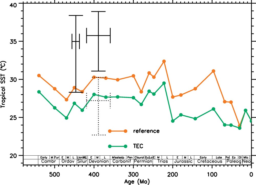
Averaged tropical sea surface temperature calculated in the reference and TEC simulations. The crosses stand for data (conodont apatite δ18O data for the Devonian, Joachimski et al., 2009 with the Pucéat et al. (2010) new paleothermometer; Δ47 data for the Ordovician from Finnegan et al., 2011). The dotted cross represents temperature for the Devonian when the Kolodny et al. (1983) paleothermometer is used.
Température moyenne des eaux tropicales de surface, calculée dans les simulations de référence et TEC. Les croix représentent les températures reconstruites à partir des données δ18O sur conodontes pour le Dévonien (Joachimski et al., 2009) (avec le paléothermomètre de Pucéat et al. (2010)), et des données Δ47 pour l’Ordovicien (Finnegan et al., 2011). La croix en pointillés représente la température moyenne pour le Dévonien, quand le paléothermomètre de Kolodny et al. (1983) est utilisé.
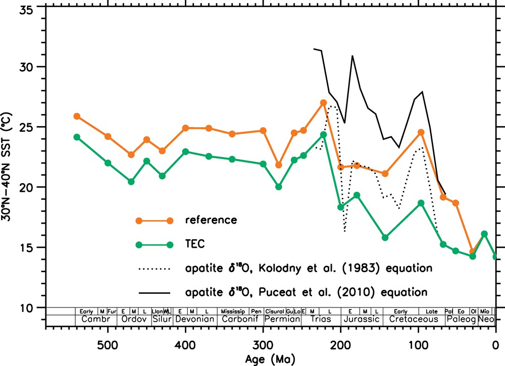
Averaged surface seawater temperatures between 30°N–40°N latitude for the reference and TEC simulations. The black lines stand for the temperatures reconstructed from apatite δ18O data, compilation by E. Pucéat (personal communication), with two different paleothermometers.
Températures moyennes d’eaux de surface entre les latitudes 30°N–40°N, calculées dans les simulations de référence et TEC. Les lignes noires montrent la température reconstruite à partir des données δ18O sur apatite sédimentaire, avec deux paléothermomètres différents (compilation par E. Pucéat, communication personnelle).
The problem may be rooted in the CO2 proxies. Indeed, as emphasized by Huber and Caballero (2011), the calibration of the leaf stomatal index method at high CO2 is weakly constrained and recent evidence that leaves adapt not only the size of the stomata but also their density at high CO2 values (Franks and Beerling, 2009) raises questions about the validity of the proxy at high CO2. Indeed, as recently affirmed by Smith et al. (2010), the stomatal methods should probably be considered semi-quantitative under high CO2 conditions and may represent CO2 minima. We also have to acknowledge that several unconstrained parameters are deeply rooted in the pedogenic carbonate method; the most critical is the fraction of below ground CO2 respired by land plants (Royer et al., 2001) for the distant geological past.
Another cause of the apparent temperature-CO2 paradox might be the model climate sensitivity. Here, the response of the mean global air temperature to a CO2 doubling is a function of the continental configuration (Fig. 9). It reaches a maximum of 4 °C during the Triassic (Pangea configuration) and when most of the continents are located around the South pole (beginning of the Phanerozoic). Then it fluctuates between 2.3 and 3 °C for other periods. Two conclusions arise from this. First, since the climate sensitivity is a function of the continental configuration, we think that using the reconstructions of past geological climates to constrain the future climate sensitivity must be undertaken with an extreme caution, particularly for the Mesozoic and Paleozoic climates (Royer et al., 2007). Park and Royer (2011) found a roughly constant sensitivity at 3 to 4 °C, except during ice ages where the sensitivity rises. Here, accounting physically for the impact of the continental configuration, the picture appears rather different: we found that the sensitivity is highest during periods characterized by supercontinental or “polar-location” configurations (where large continents are located at high latitudes), while other periods display a sensitivity at the lower band of the Park and Royer estimates. Second, the climate model used in this study has a sensitivity which is not anomalously low, given what is known of the climate behavior (Meehl et al., 2007), so that the question of the discrepancy between proxy-based temperatures and CO2 remains unsolved.
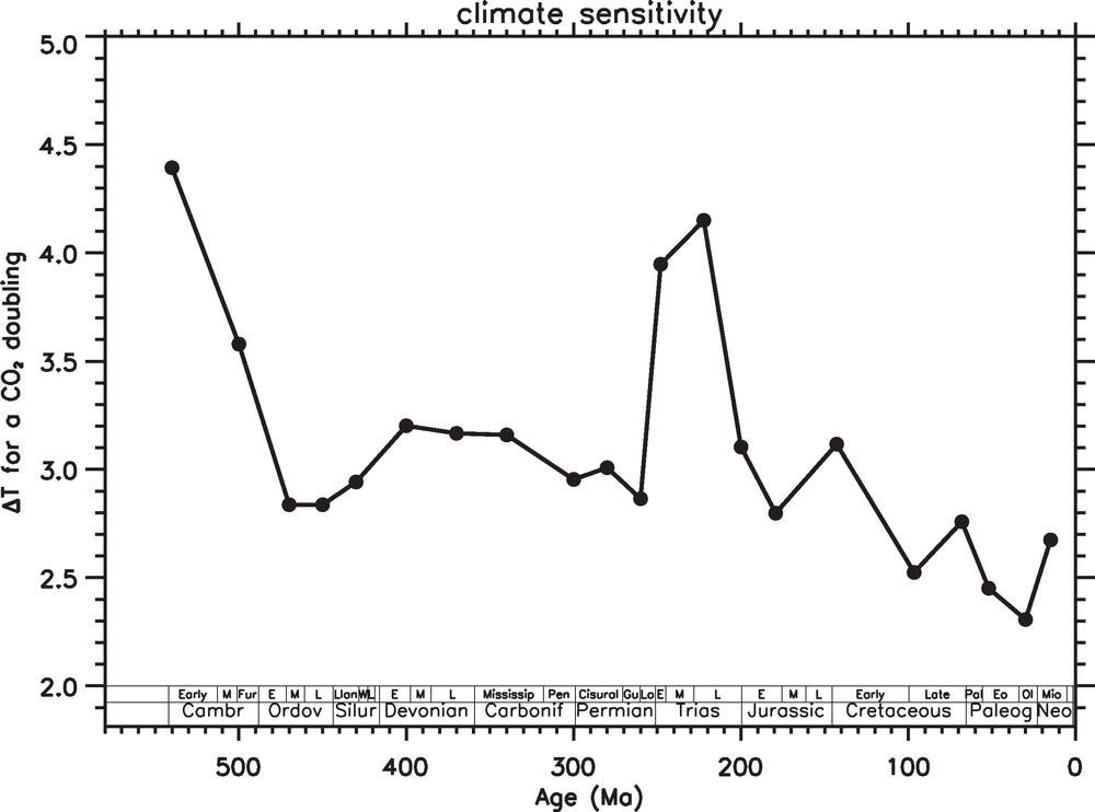
Mean global air temperature sensitivity of the FOAM climate model to a CO2 doubling as a function of the geological age.
Sensibilité de la température moyenne globale de l’air calculée par le modèle climatique FOAM à un doublement de CO2 atmosphérique, en fonction de l’âge géologique.
5 Conclusions and future research directions
In this contribution, we estimated the atmospheric CO2 levels for 21 Phanerozoic timeslices, using a coupled 3D climate and carbon-alkalinity model (GEOCLIM). Our aim was to explore the role of the tectonic drift on the time evolution of the CO2 level at the Phanerozoic timescale. Compilation of several of our previous studies in combination with new simulations, led us to suggest that the Phanerozoic tectonic drift induces a periodic climatic signal, alterning warmer and colder periods with a periodicity of about 115 Myr, in close agreement with the climatic periodicity inferred from glacial deposit inventory (Frakes et al., 1992) and from carbonate δ18O data (Veizer et al., 2000).
The paleogeographic configuration also forces the atmospheric CO2 to high levels in the Early Paleozoic and within a time window from the Late Permian to the Late Triassic. This time window is interesting. The tectonic drift may explain by itself why this period was warm, mainly because it was dry, a state inhibiting CO2 consumption by continental weathering. Although this warm interval is recorded in many climatic indexes, including δ18O data (Prokoph et al., 2008; Veizer et al., 2000), it is totally absent from the CO2 proxy-based curve. This particular case illustrates a general discrepancy existing between the proxy-based CO2 levels and the reconstructed Phanerozoic climates. The proxy-based CO2 levels are generally too low to explain the observed climatic features.
One last conclusion is that the distant past might not be the key to the future. We show that the climate sensitivity to atmospheric CO2 depends on the paleogeographic configuration, being maximal (4 °C for a CO2 doubling) during supercontinental configurations or when continents are mostly located at high latitudes.
In the future, similar studies should be performed with other general circulation models. We must be aware that the vast majority of deep time climatic studies were performed with the GENESIS GCM, while we used another 3D FOAM GCM climate model. Each of these models has its own limitations. For climate studies dealing with the future evolution of the Earth system, the Intergovernmental Panel on Climate Change (IPCC) uses a large variety of models in order to estimate the inherent uncertainties (Meehl et al., 2007) and we believe that such a procedure should be employed also for the study of the coupled evolution of the carbon cycle and climate in the past.
Acknowledgements
Funding for this study has been provided by the INSU/CNRS through the Eclipse and SYSTER programs, and by the National Agency for Research projects ACCRO-Earth (ANR-06-BLAN-0347) and COLORS (ANR-09-JCJC-0105). We thank Bob Berner for helpful discussions and for comments on an early version of this manuscript. Continental configurations have been provided by R.C. Blakey for the Paleozoic, and by F. Fluteau, J. Sewall and N. Herold for the Mesozoic and Cenozoic. We thank R.T. Pierrehumbert, G. Ramstein, E. Pucéat for helpful discussions over the last few years.