Seismic random noise attenuation and signal-preserving by multiple directional time-frequency peak filtering

Chao Zhang; Yue Li; Hong-bo Lin; Bao-jun Yang

doi:10.1016/j.crte.2014.10.003

Internal geophysics

Seismic random noise attenuation and signal-preserving by multiple directional time-frequency peak filtering

Chao Zhang ¹ ; Yue Li ¹ ; Hong-bo Lin ¹ ; Bao-jun Yang ²

¹ Department of Information, College of Communication Engineering, Jilin University, Changchun 130012, China
² Department of Geophysics, Jilin University, Changchun 130026, China

Comptes Rendus. Géoscience, Volume 347 (2015) no. 1, pp. 2-12.

Résumé

Time-frequency peak filtering (TFPF) is an effective method for seismic random noise attenuation. The linearity of the signal has a significant influence on the accuracy of the TFPF method. The higher the linearity of the signal to be filtered is, the better the denoising result is. With this in mind, and taking the lateral coherence of reflected events into account, we do TFPF along the reflected events to improve the degree of linearity and enhance the continuity of these events. The key factor to realize this idea is to find the traces of the reflected events. However, the traces of the events are too hard to obtain in the complicated field seismic data. In this paper, we propose a Multiple Directional TFPF (MD–TFPF), in which the filtering is performed in certain direction components of the seismic data. These components are obtained by a directional filter bank. In each direction component, we do TFPF along these decomposed reflected events (the local direction of the events) instead of the channel direction. The final result is achieved by adding up the filtering results of all decomposition directions of seismic data. In this way, filtering along the reflected events is implemented without accurately finding the directions. The effectiveness of the proposed method is tested on synthetic and field seismic data. The experimental results demonstrate that MD–TFPF can more effectively eliminate random noise and enhance the continuity of the reflected events with better preservation than the conventional TFPF, curvelet denoising method and F–X deconvolution method.

Métadonnées

Reçu le : 2014-08-18
Accepté le : 2014-10-16
Publié le : 2014-12-08

DOI : 10.1016/j.crte.2014.10.003

Mots clés : Time-frequency peak filtering, Directional filter bank, Resampling, Random noise attenuation

Affiliations des auteurs :

Chao Zhang ¹ ; Yue Li ¹ ; Hong-bo Lin ¹ ; Bao-jun Yang ²

¹ Department of Information, College of Communication Engineering, Jilin University, Changchun 130012, China
² Department of Geophysics, Jilin University, Changchun 130026, China

@article{CRGEOS_2015__347_1_2_0,
     author = {Chao Zhang and Yue Li and Hong-bo Lin and Bao-jun Yang},
     title = {Seismic random noise attenuation and signal-preserving by multiple directional time-frequency peak filtering},
     journal = {Comptes Rendus. G\'eoscience},
     pages = {2--12},
     publisher = {Elsevier},
     volume = {347},
     number = {1},
     year = {2015},
     doi = {10.1016/j.crte.2014.10.003},
     language = {en},
}

TY  - JOUR
AU  - Chao Zhang
AU  - Yue Li
AU  - Hong-bo Lin
AU  - Bao-jun Yang
TI  - Seismic random noise attenuation and signal-preserving by multiple directional time-frequency peak filtering
JO  - Comptes Rendus. Géoscience
PY  - 2015
SP  - 2
EP  - 12
VL  - 347
IS  - 1
PB  - Elsevier
DO  - 10.1016/j.crte.2014.10.003
LA  - en
ID  - CRGEOS_2015__347_1_2_0
ER  -

%0 Journal Article
%A Chao Zhang
%A Yue Li
%A Hong-bo Lin
%A Bao-jun Yang
%T Seismic random noise attenuation and signal-preserving by multiple directional time-frequency peak filtering
%J Comptes Rendus. Géoscience
%D 2015
%P 2-12
%V 347
%N 1
%I Elsevier
%R 10.1016/j.crte.2014.10.003
%G en
%F CRGEOS_2015__347_1_2_0

Chao Zhang; Yue Li; Hong-bo Lin; Bao-jun Yang. Seismic random noise attenuation and signal-preserving by multiple directional time-frequency peak filtering. Comptes Rendus. Géoscience, Volume 347 (2015) no. 1, pp. 2-12. doi : 10.1016/j.crte.2014.10.003. https://comptes-rendus.academie-sciences.fr/geoscience/articles/10.1016/j.crte.2014.10.003/

Version originale du texte intégral

1 Introduction

The reflected events contained in the seismic data play an important role in the study of geological structures. However, the noise contamination corrupts the quality of the reflected events and disturbs the identification of geological information. Therefore, the noise attenuation is crucial to seismic data analysis (Klemperer and Brown, 1985; Zhang and Klemperer, 2005; Zhang and Ulrych, 2003). Usually, random noise can be generated during data acquisition by various sources and this noise is unpredictable in space and time. So, it is difficult to remove random noise from the seismic data. In recent years, many efforts have been made for seismic random noise attenuation (e.g., Abma and Claerbout, 1995; Cao and Chen, 2005; Jones and Levy, 2006; Wang, 1999, 2002). However, most of the existing denoising methods do not work well in the case of low signal-to-noise ratios (SNRs). It performs poorly in signal preservation, which leads to a decline of the fidelity in seismic data processing. Thus, one of the tasks is to design a denoising method to balance the noise attenuation and signal preservation, especially when the SNR is low.

TFPF is a one-dimensional (1-D) time-frequency filtering algorithm. It can give an unbiased estimation where the signal is linear in time and embedded in white Gaussian noise (Barkat and Boashash, 1999; Boashash and Mesbah, 2004; Zahir and Hussain, 2002). It has been successfully applied to the seismic data processing field (Li et al., 2009; Lin et al., 2007, 2013; Zhang et al., 2013). This method enhances non-stationary signals from random noise through frequency modulation and instantaneous frequency estimation by taking the peak in the time-frequency distribution. In general, we use pseudo Wigner–Ville distribution (PWVD) to realize local linearity. The unbiased estimation condition of the TFPF can be better satisfied if the signal has a high degree of linearity. The nonlinearity of signals will result in amplitude loss in the TFPF. So how to increase the linearity is crucial to the TFPF. One of the effective solutions is to filter along the reflected events. It also takes the coherence between the adjacent channels into consideration, which has a positive effect on the continuity of reflected events. With this in mind, an improved TFPF algorithm has been developed and filtering along a radial trace with an angle to the channel direction (Wu et al., 2011). However, a fixed radial filtering trace cannot fit with the curve reflected events effectively, which leads to some limitations in actual application. A similar trace to the reflected events for filtering is important (Tian and Li, 2014), but the field seismic data is too complicated to find a suitable trace for all the reflected events.

This paper introduces a Multiple Directional Time-Frequency Peak Filtering technique. To do the TFPF along the reflected events, we decompose the 2-D matrix of seismic data into multiple direction components. The direction decomposition is equivalent to the use of some linear segments to approximate the curve reflected events. The distributions of the events in each direction component show as the straight line and have the same slope; the slope direction is the direction of decomposition. So, TFPF could be done along a group of parallel radial filtering traces with the same slope as the decomposed reflected events in each direction component. The sum of the filtering results from all the given directions as the final processed result. The direction decomposition is realized using the directional filter bank. Our method makes the filtering along the reflected events possible by a novel idea without finding the accurate traces of all the reflected events.

2 Time-frequency peak filtering

Let the noisy signal $s (t)$ be modeled by the equation:

s (t) = x (t) + n (t),

(1)

where

x (t)

is the band-limited non-stationary deterministic signal and

n (t)

is the random noise. The goal of this algorithm is to recover the signal x(t) from the observed signal s(t). TFPF extracts the valid signal in the following steps (Boashash and Mesbah, 2004).

First, we encode the noisy signal $s (t)$ as the instantaneous frequency of the analytic signal $z_{s} (t)$ via frequency modulation; $z_{s} (t)$ can be expressed as:

z_{s} (t) = e^{j 2 π μ \int_{0}^{t} s (λ) d λ},

(2)

where

μ

is a scaling parameter analogous to the frequency modulation index.

Then we calculate the Wigner–Ville distribution (WVD) of the analytic signal $z_{s} (t)$ through

W V D_{z_{s}} (t, f) = \int_{- \infty}^{\infty} z_{s} (t + τ / 2) {z_{s}}^{*} (t - τ / 2) e^{- j 2 π f τ} d τ,

(3)

where

t

and

f

are the time and frequency variables, respectively.

Finally, we estimate the peak of $W V D_{z_{s}} (t, f)$ to obtain the instantaneous frequency of z_s(t). Since we encode the noisy signal s(t) as the instantaneous frequency of z_s(t) by Eq. (2), the estimated instantaneous frequency is the estimation of the signal x(t), which is expressed as:

\hat{x} (t) = \underset{f}{\arg max} [W V D_{z_{s}} (t, f)] / μ .

(4)

where

\hat{x} (t)

denotes the estimation of the signal

x (t)

{\hat{f}}_{z_{s}} (t)

is the estimated instantaneous frequency of

z_{s} (t)

The TFPF method is unbiased for a linear signal $x (t) = α t + C$ ( $α$ and C are constants) from white Gaussian noise. The bias B(t) is defined as $B (t) = E [\hat{x} (t) - x (t)]$ , E denotes the mathematical expectation. If a signal is embedded in a stationary white Gaussian noise background, the final derivation result of the bias $B (t)$ of the TFPF algorithm is written as (Boashash and Mesbah, 2004):

B (t) = \underset{f}{\arg m a x} (W V D_{z_{x}} (t, f) \underset{f}{\times} {(4 π^{2} k_{n_{2}} μ^{2} / ((2 π^{2} k_{n_{2}} μ^{2})}^{2} + {(2 π f)}^{2}))) - x (t),

(5)

where

W V D_{z_{s}} (t, f)

denotes the WVD of

z_{x} (t)

as Eq. (3) and

k_{n_{2}}

is the second cumulant of the noise

n (t)

. For the case where the signal

x (t)

is linear in time,

B (t)

become:

\begin{array}{l} B (t) = \underset{f}{\arg m a x} (δ (f - x (t)) \underset{f}{*} (4 π^{2} k_{n_{2}} μ^{2} / ({(2 π^{2} k_{n_{2}} μ^{2})}^{2} + {(2 π f)}^{2}))) - x (t) \\ = \underset{f}{\arg m a x} (4 π^{2} k_{n_{2}} μ^{2} / ({(2 π^{2} k_{n_{2}} μ^{2})}^{2} + {(2 π (f - x (t)))}^{2})) - x (t) = 0. \end{array}

(6)

Equations (6) are derived in the case of stationary white Gaussian noise. However, the analysis can also be applied to other types of noise as long as the signal

x (t)

is linear in time because the

B (t)

in Eq. (5) is independent of the

k_{n_{2}}

of the noise. Hence, if the signal is linear in time, TFPF can give an unbiased estimation.

However, the reflected seismic signals are nonlinear. So, there must be a bias in the filtering processing by the TFPF. To reduce the bias, TFPF adopts the PWVD, which is the windowed version of the WVD to make the signal approximately linear within the window. The PWVD is defined as (Barbarossa, 1997):

P W V D_{z} (t, f) = \int_{- \infty}^{\infty} h (τ) z (t + τ / 2) z^{*} (t - τ / 2) e^{- j 2 π f τ} d τ,

(7)

where

h (τ)

is a window function sliding with time.

The PWVDs of an analytic Ricker wavelet contaminated by an additive white Gaussian noise (SNR = 0 dB) are shown on Fig. 1. On this illustration, we can see that the peak of the PWVD is mainly located at the instantaneous frequency of the analytic signal. So, we can use the peak of the PWVD to recover the reflected signal.

Fig. 1
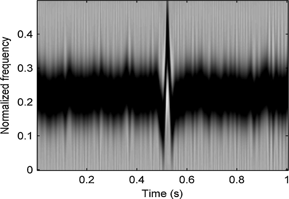
Pseudo Wigner–Ville distribution of a Ricker wavelet contaminated by additive white Gaussian noise (signal-to-noise ratio = 0 dB).

3 Principle of multiple directional TFPF

To obtain an unbiased result, one effective way is to improve the degree of linearity of the desired signal, which is an unbiased estimation condition of TFPF. The solution can be implemented by filtering along the reflected events. Fig. 2b shows five representative radial traces corresponding to the numbered trajectories on Fig. 2a (Wu et al., 2011). We can see that a common-origin seismic reflected event can be mapped into a comparatively higher degree of linearity when the slope of the trajectory is close to that of the event. So, the radial traces such as direction 1 or 2 are suitable for the unbiased TFPF because the signals extracted from these radial traces have a much higher degree of linearity. Thus, constructing the reasonable filtering traces of events is the key of TFPF method to reduce the bias. However, the traces suitable for all the reflected events in the field data are too difficult to construct because of complexity and noise interference. However, we may change our idea to implement trace construction for all the reflected events by decomposing the seismic reflected events into some linear segments. In other words, we use some linear segments to approximate the events. Then, TFPF can be done along multiple linear segments that are the local direction of events reflected by a group of parallel radial filtering traces. Considering that the linear segmentation is difficult to realize in the time domain, we can perform the decomposition in the frequency domain. The spectrum of the noisy synthetic seismic record (Fig. 3a) in the frequency-wavenumber domain is shown on Fig. 3b. We divide the region with energy distribution into some directions. The direction division in the frequency domain is equivalent to approximating the events by some linear segments in the time domain. The more directions we divide in frequency domain, the higher the linearity of local reflected events in each direction component is. In other words, if the curvature of reflected events is larger, more linear segments are used to approximate the events so that we can do filtering along the local reflected events by a group of parallel radial filtering traces.

Fig. 2
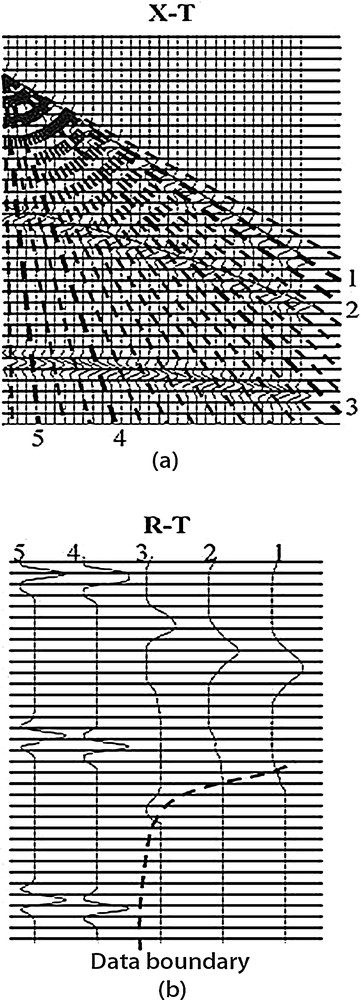
a: Radial traces on a seismic panel; b: representative radial traces extracted from the seismic panel.

Fig. 3
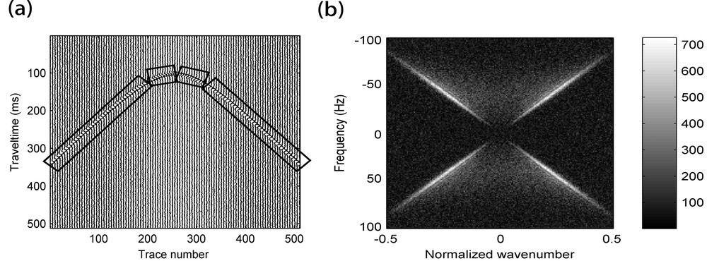
a: A noisy synthetic seismic record (signal-to-noise ratio = –5 dB) with a hyperbolic reflected event. The dominant frequency of the event is 30 Hz. The source wavelet we applied to simulate the waveform is Ricker wavelet; b: the spectrum of Fig. 3a in the frequency–wavenumber domain.

These direction components are obtained by a 2-D directional filter bank. This directional filter bank can decompose a 2-D matrix of seismic data according to directions while achieving perfect reconstruction (Do and Vetterli, 2005; Feilner et al., 2005). The directional filter bank is efficiently implemented via an l-level binary tree decomposition that leads to $2^{l}$ sub-bands with wedge-shaped frequency partitioning. The decomposition of a noisy seismic data $s (n)$ of time-offset domain $(n = (d, t), d is offset)$ by the directional filter bank can be written as:

s (n) = \sum_{k} s_{k} (n) = \sum_{k = 0}^{2^{l} - 1} \sum_{m \in Z^{2}} y_{k} (m) g_{k} (n - S_{k} m),

(8)

where

y_{k} (m) \leq s (n), h_{k} (S_{k} m - n) >,

(9)

with

S_{k}

the sampling matrices that have the following diagonal forms (Do and Vetterli, 2005)

S_{k} = \{\begin{array}{l} d i a g (2^{l - 1}, 2) f o r 0 \leq k < 2^{l - 1}, \\ d i a g (2, 2^{l - 1}) f o r 2^{l - 1} \leq k < 2^{l}, \end{array}

(10)

$s_{k} (n)$ is a decomposed direction component of $s (n)$ and $k$ the direction index. $h_{k} (n)$ is the impulse response of analysis filter and $g_{k} (n)$ is the impulse response of synthesis filters. $m$ is used to denote location of noisy seismic data.

Next we give the whole filter process of our multiple directional TFPF. First, we decompose a noisy seismic data $s (d, t)$ into some direction components by Eq. (8). Each decomposed component $s_{k} (d, t)$ has its own orientation depending on the index $k$ . We take the noisy synthetic seismic record (Fig. 3a) as an example. The decomposed direction components of Fig. 3a are shown on Fig. 4.

Fig. 4
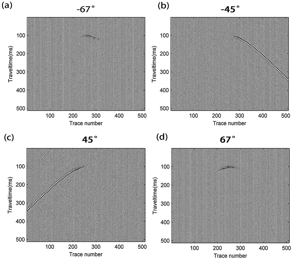
Direction decomposition of a noisy synthetic seismic record (signal-to-noise ratio = –5 dB) with a hyperbolic reflected event: a–d: the different direction components of the seismic data that are decomposed by a directional filter bank (DFB).

Then the data in each component need to be resampled along this known decomposed direction. The processing can be realized by transforming a 2-D matrix of seismic data into a new data matrix along some parallel traces in this decomposed direction. The corresponding multiple directional filtering traces are shown on Fig. 5. The equation of the parallel trace that we used is expressed as

t_{i} = a_{k} d_{i} + b .

(11)

where

a_{k}

is defined as the slope in the direction

k

;

b

is the intercept. In the process of data resampling,

d_{i}

corresponds to the channel and

t_{i}

corresponds to the data sample point. To extract sample points along the parallel trace, we should find the horizontal and vertical coordinates of each sample point on the parallel trace. Taking time as the vertical coordinate, we can find the corresponding horizontal coordinate of each time point t_i according to Eq. (11). After resampling, the new data matrix in each direction component is filtered by the TFPF method.

Fig. 5
Filtering traces in different decomposed directions: a–d: filtering traces in the directions that correspond to Fig. 4.

The parameter $a_{k}$ denotes the direction of filtering method. Our method applies the TFPF along different $a_{k} - directions,$ which are also the decomposition directions of the reflected events. The final result is obtained by putting the filtering results from all the directions of reflected events together. The effect of the whole processing is equivalent to the filtering along seismic reflected events and avoids finding the directions of all the events.

4 Implementation and applications

4.1 Synthetic data example

To verify the effectiveness of the proposed MD–TFPF, we gave it to process synthetic seismic data. The synthetic example is a seismic model with three hyperbolic reflected events as shown on Fig. 6a. We add a white Gaussian noise to the synthetic model. Fig. 6b is a noisy version (SNR = −5 dB) of the noise-free Fig. 6a. In this example, MD–TFPF is compared with conventional TFPF. Fig. 6c and d show the denoising results by the two methods. As can be seen from Fig. 6c and d, we can achieve the visual qualitative performance. Both two methods can suppress some random noise and the three events can be identified. While the MD–TFPF achieves clean background and the reflected events are continuous and recovered, especially in the rectangular region.

Fig. 6
Denoising with synthetic seismic data: a: synthetic seismic data. Three Ricker wavelets of dominant frequencies 25, 30, and 35 Hz were considered to simulate synthetic waveforms as natural events; b: noisy seismic data (signal-to-noise ratio = –5 dB). The synthetic data were contaminated with white Gaussian noise; c: result after applying conventional TFPF; d: result after applying multiple directional–time-frequency peak filtering (MD–TFPF); e: comparison of results after processing a single synthetic trace (36th trace) with both filtering types for noise suppression. The ideal signal is plotted with a dotted line and the solid line represents the filtered signal; f: amplitude spectrum of the original signal and the two filtered signals. The ideal spectrum is plotted with a dotted line and the solid line represents the filtered spectrum of the signal.

Detailed effects of the two processing consequents can be obtained by analyzing the single trace and its amplitude spectrum. We extract the 36th trace of the synthetic records and redisplay it as an example. The amplification waveforms in time and frequency domains are shown on Fig. 6e and f. Fig. 6e exhibits the denoising result of a seismic wavelet from the 36th trace of the synthetic record in the time domain. Notice that the filtering result of MD–TFPF is close to the original signal and the amplitude value of noise on both sides of the signal is significantly lower than conventional TFPF does. Through the calculation, the correlation coefficient between the original signal and the denoised signal by using MD–TFPF is up to 0.83, but using a conventional TFPF method, the correlation coefficient is only 0.54. Furthermore, we also compare the filtering performance in the frequency domain, which is shown on Fig. 6f. It can also be seen that the MD–TFPF provides the best-matching amplitude spectrum to the noise-free spectrum for the signal components in the 0–70 Hz band. The spectrum of the convention TFPF has larger high-frequency components after 70 Hz than our method. So the random noise is effectively suppressed.

In the following, we ran extensive tests on data with white Gaussian noise at different levels to show the effectiveness of the MD–TFPF on SNR (in dB) and mean square error (MSE).

Table 1 gives the resulting SNR and MSE for synthetic seismic data of Fig. 6a. The better ﬁltering effect has larger SNR value and lower MSE value. As can be seen in Table 1, the SNRs after filtering by the MD–TFPF are larger and the MSEs are smaller than when applying conventional TFPF in any SNR. This advantage of the MD–TFPF is obvious when the SNR is below −8 dB. The result implies that MD–TFPF provides accurate estimation and improvement to noisy signals.

SNR (in dB) computed from the original signal	Processed signal by conventional TFPF	Processed signal by MD–TFPF
	SNR (dB)	MSE	SNR (in dB)	MSE
−20	−13.21	0.8652	−10.56	0.4283

−16	−9.83	0.6831	−5.33	0.2946

−12	−6.1	0.4314	−1.46	0.1887

−8	−1.16	0.3427	2.78	0.1153

−4	3.24	0.2135	5.92	0.0832

0	7.86	0.1682	9.32	0.0667

4	9.17	0.1026	12.29	0.0465

8	12.93	0.0868	14.45	0.0329

Our method has another advantage, which is that it can recover signals from non-stationary random noise with very low SNR. We add a non-stationary random noise with high noise levels to the synthetic model (Fig. 6a). The noisy record with the SNR −15 dB is shown on Fig. 7a, where the three hyperbolic reflection events are almost submerged completely in the strong noise. In this example, the MD–TFPF is compared with conventional TFPF and the curvelet denoising method. Fig. 7b, c and d show the denoising results by curvelet denoising method, conventional TFPF and our method, respectively. Notice that the events on Fig. 7b and c can hardly be identified while they are well recovered on Fig. 7d. Thus, the MD–TFPF is also very effective in the low SNR.

Fig. 7
The filtering results of synthetic seismic data with low signal-to-noise ratio (SNR): a: noisy seismic data (SNR = –15 dB). The synthetic data were contaminated with non-stationary random noise; b: result after applying a curvelet denoising method; c: result after applying conventional TFPF; d: result after applying multiple directional–time-frequency peak filtering (MD–TFPF).

4.2 Field data application

A common shot point seismic data that we test is shown on Fig. 8a. The receiver interval is 30 m and the sampling frequency is 1000 Hz. The distance between the source and the receivers changes from 600 to 3600 m. The continuities of seismic reflected events are badly damaged and the events are obscured because of the interference from random noise. To show the effectiveness of our method, we compare the results of MD–TFPF with conventional TFPF and F–X deconvolution methods. It can be found that F–X deconvolution (Fig. 8b) and conventional TFPF methods (Fig. 8c) cannot reduce random noise as effectively as MD–TFPF, whose results are displayed on Fig. 8d, particularly in the ellipse area. To demonstrate the visual quality of the events, we show an enlarged view between traces 60–110 and double-time 500–1200 ms (Fig. 9) in the rectangle on Fig. 8. In contrast, the reflected events processed by MD–TFPF (Fig. 9d) are clearly recovered and the events continuity is enhanced (e.g., in the rectangles). According to the experimental results, the proposed MD–TFPF method has a great advantage in eliminating random noise and efficiently protecting the reflected events compared with the other two methods.

Fig. 8
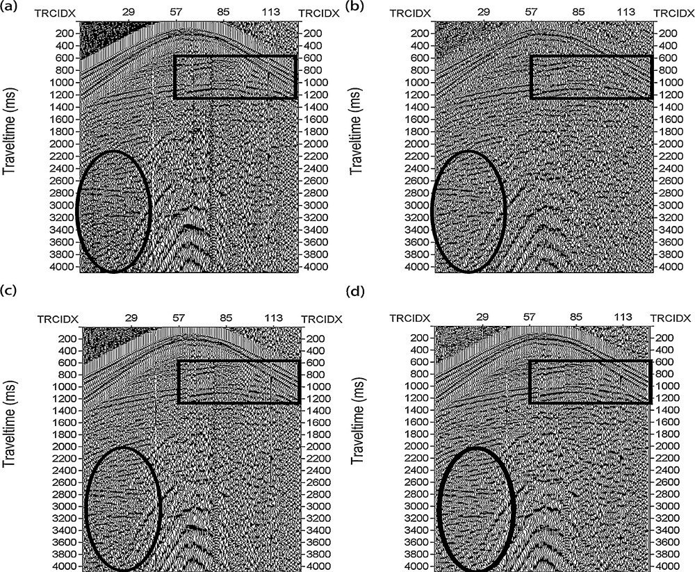
Results obtained with field seismic data: a: field seismic data (common shot point seismic data); b: result after applying the F–X deconvolution method; c: result after applying conventional TFPF; d: result after applying the multiple directional–time-frequency peak filtering (MD–TFPF). Ellipses and rectangles delimit those areas where we can observe better the progressive efficiency of denoising and signal preservation, respectively.

Fig. 9
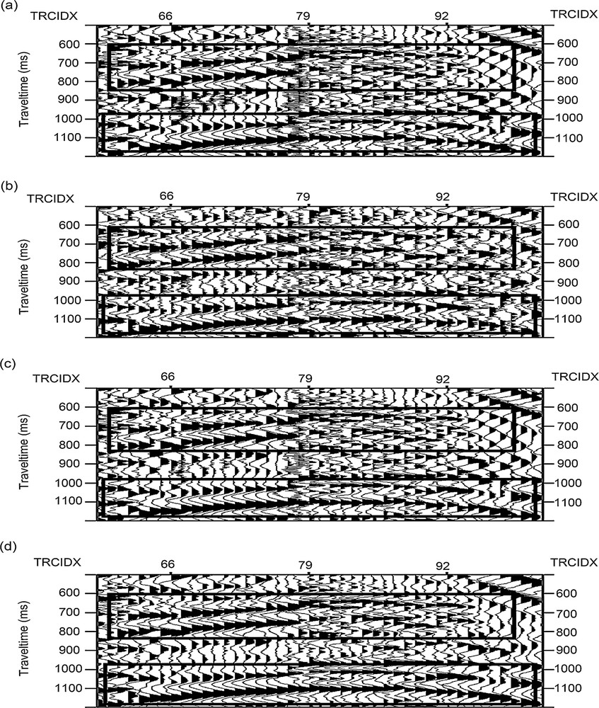
An enlarged view allowing seeing the quality of the filtering between the traces 60 to 110 and double travel times from 500 to 1200 ms: a: unfiltered zoomed record; b: filtered zoomed record using the F–X deconvolution method; c: filtered zoomed record using conventional TFPF; d: filtered zoomed record using multiple directional–time-frequency peak filtering (MD–TFPF).

We also apply our method to a real seismic section to test the applicability. Fig. 10a shows a section with high background random noise. This background random noise overwhelms weak reflected events and disrupts the continuity of events over the entire section. We compare the MD–TFPF with conventional TFPF and the curvelet denoising method. As seen on Fig. 10b and c, some random noise still exists after filtering by curvelet denoising method and conventional TFPF method, especially in the rectangular region. However, the application of MD–TFPF method shows that most of the background noise is suppressed without the edges of the reflected events being blurred and the method does not make any significant changes to the shapes of reflected events. Furthermore, the weak reflected events continuity is also enhanced. This method greatly improved SNR, which is clearly identified on the seismic section (Fig. 10d). The result on Fig. 10d shows that even with strong random noise, the proposed method is still effective in suppressing noise.

Fig. 10
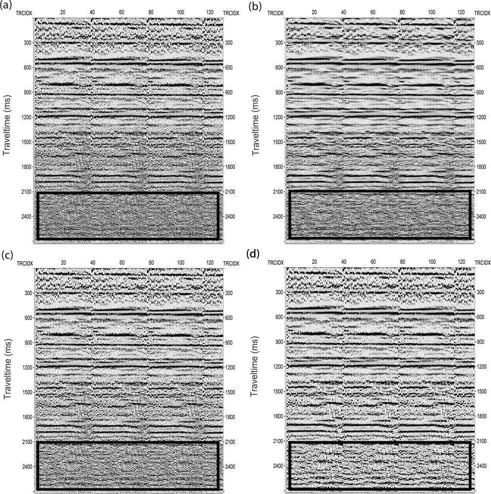
Filtering results of real seismic section with low signal-to-noise ratio: a: seismic section; b: result after applying the curvelet denoising method; c: result after applying conventional TFPF; d: result after applying the multiple directional–time-frequency peak filtering (MD–TFPF). We can see better the progressive efficiency of denoising and signal preservation in the rectangles.

5 Conclusions

In this paper, a multiple directional time-frequency peak filtering has been proposed to improve the filtering result in the conventional time-frequency peak filtering. It filters the seismic data along multiple decomposed directions of the reflected events instead of the channel direction. The coherence between adjacent channels is fully considered and utilized, which recovers the reflected events more clearly and continuously. The direction decomposition is realized based on a directional filter bank. In this novel method, the directions of reflected events are indirectly obtained by a directional filter bank without accurately tracing all the events, which makes filtering along the reflected events in the complex field seismic data possible. Therefore, our method has a high practicability in seismic data denoising. Texts on both synthetic and field seismic data have demonstrated that the proposed method can preserve signals and effectively enhance the continuity of reflected events. Furthermore, the proposed method makes it possible to recover the desired seismic signal in the case of SNR down to −15 dB. It has great practical value, especially when the SNR of seismic data is very low.

Acknowledgments

This research is financially supported by the National Natural Science Foundation of China (under grants 41130421 and 41274118); Science and Technology Development program of Jilin Province of China (under grant 20110362) and the Development and Reform Commission of Jilin Province (grants No. 2011006-2, JF2012C013-2).

Bibliographie

[Abma and Claerbout, 1995] R. Abma; J. Claerbout Lateral prediction for noise attenuation by T–X and F–X techniques, Geophysics, Volume 60 (1995), pp. 1887-1896

[Barbarossa, 1997] S. Barbarossa Parameter estimation of spread spectrum frequency hopping signals using time-frequency distributions, First IEEE Signal Processing Workshop on Signal Processing Advances in Wireless Communications, 1997, pp. 213-216

[Barkat and Boashash, 1999] B. Barkat; B. Boashash Design of higher order polynomial Wigner-Ville distributions, IEEE Trans. Signal Process., Volume 47 (1999), pp. 2608-2611

[Boashash and Mesbah, 2004] B. Boashash; M. Mesbah Signal enhancement by time-frequency peak filtering, IEEE Trans. Signal Process., Volume 52 (2004), pp. 929-937

[Cao and Chen, 2005] S.Y. Cao; X.P. Chen The second generation wavelet transform and its application in denoising of seismic data, Appl. Geophys., Volume 2 (2005), pp. 70-74

[Do and Vetterli, 2005] M.N. Do; M. Vetterli The contourlet transform: an efficient directional multiresolution image representation, IEEE Trans. Image Process., Volume 14 (2005), pp. 2091-2106

[Feilner et al., 2005] M. Feilner; D.D. Ville; M. Unser An orthogonal family of quincunx wavelets with continuously adjustable order, IEEE Trans. Image Process., Volume 14 (2005), pp. 499-510

[Jones and Levy, 2006] I.F. Jones; S. Levy Signal-to-noise ratio enhancement in multichannel seismic data via the Karhunen-Loeve transform, Geophys. Prospect., Volume 35 (2006), pp. 12-32

[Klemperer and Brown, 1985] S.L. Klemperer; L. Brown Simulations of noise rejection and mantissa-only recording; an experiment in high-amplitude noise reduction with COCORP data, Geophysics, Volume 50 (1985), pp. 709-714

[Lin et al., 2007] H.B. Lin; Y. Li; B.J. Yang Recovery of seismic events by time-frequency peak filtering, IEEE International Conference on Image Processing, 2007, pp. 441-444

[Lin et al., 2013] H.B. Lin; Y. Li; B.J. Yang; H.T. Ma Random denoising and signal nonlinearity approach by time-frequency peak filtering using weighted frequency reassignment, Geophysics, Volume 78 (2013), pp. 229-237

[Li et al., 2009] Y. Li; H.B. Lin; B.J. Yang; N. Wu; S.K. Li; H. Gao The influence of limited linearization of time window on TFPF under the strong noise background, Chin. J. Geophys., Volume 52 (2009), pp. 1899-1906 (in Chinese)

[Tian and Li, 2014] Y.N. Tian; Y. Li Parabolic-trace time-frequency peak filtering for seismic random noise attenuation, IEEE Geosci. Remote Sens. Lett., Volume 11 (2014), pp. 158-162

[Wang, 1999] Y. Wang Random noise attenuation using forward-backward linear prediction, J. Seism. Explor., Volume 8 (1999), pp. 133-142

[Wang, 2002] Y. Wang Seismic trace interpolation in the f–x–y domain, Geophysics, Volume 67 (2002), pp. 1232-1239

[Wu et al., 2011] N. Wu; Y. Li; B.J. Yang Noise attenuation for 2-D seismic data by radial trace time-frequency peak filtering, IEEE Geosci. Remote Sens. Lett., Volume 8 (2011), pp. 874-878

[Zahir and Hussain, 2002] M. Zahir; B. Hussain Adaptive instantaneous frequency estimation of multicomponent FM signal using quadratic time-frequency distributions, IEEE Trans. Signal Process., Volume 50 (2002), pp. 657-660

[Zhang et al., 2013] C. Zhang; H.B. Lin; Y. Li; B.J. Yang Seismic random noise attenuation by time-frequency peak filtering based on joint time-frequency distribution, C. R. Geoscience, Volume 345 (2013), pp. 383-391

[Zhang and Ulrych, 2003] R. Zhang; T.J. Ulrych Physical wavelet frame denoising, Geophysics, Volume 68 (2003), pp. 225-231

[Zhang and Klemperer, 2005] Z.J. Zhang; S.L. Klemperer West–east variation in crustal thickness in northern Lhasa block central Tibet, from deep seismic sounding data, J. Geophys. Res., Volume 110 (2005), p. B0943

Commentaires - Politique

Ces articles pourraient vous intéresser

Seismic random noise attenuation by time-frequency peak filtering based on joint time-frequency distribution

Chao Zhang; Hong-bo Lin; Yue Li; ...

C. R. Géos (2013)

Trace-transform-based time-frequency filtering for seismic signal enhancement in Northeast China

Ning Wu; Yue Li; Yanan Tian; ...

C. R. Géos (2016)

Seismic random noise elimination according to the adaptive fractal conservation law

Fanlei Meng; Yue Li; Qian Zeng

C. R. Géos (2016)