

1 Introduction
Geostatistical simulation is widely used in the evaluation of mineral resources and ore reserves to map geological heterogeneity at different spatial scales and to assess the uncertainty in the unknown values of coregionalized variables, such as the grades of elements of interest, petrophysical properties of the subsoil, or geometallurgical properties (work index, acid consumption, metal recoveries) (Boisvert et al., 2013; Rossi and Deutsch, 2014). Its practical implementation requires specifying a stochastic model, which describes the spatial distribution of the coregionalized variables (what should be simulated), and an algorithm, which aims at constructing realizations of the prescribed model (how it should be simulated) (Chilès and Delfiner, 2012; Lantuéjoul, 2002).
When the coregionalized variables can be modeled (up to some nonlinear transformation) by Gaussian random fields, a few exact algorithms, such as the matrix decomposition (Davis, 1987, Myers, 1989), discrete spectral (Chilès and Delfiner, 1997; Dietrich and Newsam, 1993; Le Ravalec et al., 2000 Pardo-Igúzquiza and Chica-Olmo, 1993) and moving average (Black and Freyberg, 1990) algorithms, perfectly reproduce their joint distribution and spatial correlation structure, but such algorithms are limited, either because they cannot be used for large-scale problems or because they require the data and target locations to be regularly spaced.
To overcome these limitations, approximate algorithms can be applied, allowing dealing with large numbers of data on unstructured grids. In this category, one finds the sequential Gaussian (Deutsch and Journel, 1998), continuous spectral (Shinozuka and Jan, 1972) and turning bands (Matheron, 1973) algorithms. Sequential Gaussian simulation has been widely use in practice due to its simplicity and straightforwardness in a variety of areas (Alabert and Massonnat, 1990; Ravenscroft, 1994), but the accuracy of this method is not always ensured (Emery, 2004; Emery and Peláez, 2011; Gómez-Hernández and Cassiraga, 1994; Omre et al., 1993; Tran, 1994) and its applicability to multivariate cases may be challenging and require simplifications (Almeida and Journel, 1994; Gómez-Hernández and Journel, 1993). An alternative to obtain good-quality realizations is the turning bands approach proposed by Matheron (1973). In a nutshell, this method performs simulation in a multi-dimensional space through a series of one-dimensional simulations. The algorithm allows fast calculations and, in theory, yields an accurate reproduction of the spatial correlation structure (in univariate and multivariate cases), although the resulting distributions may slightly differ from the target ones due to the use of a finite number of one-dimensional simulations (stripping effect) (Emery and Lantuéjoul, 2006).
The purpose of this paper is to assess the performance and check the accuracy of sequential Gaussian and turning bands simulation, through actual and synthetic case studies.
2 Theory of joint simulation
It is often of interest to construct numerical models that reproduce the joint distribution of several coregionalized variables at unsampled locations, conditionally to the information available at sampling locations (conditional cosimulation). Because the variables are usually spatially cross-correlated, it is not sufficient to simulate each variable separately. Instead, a multivariate approach has to be used.
In the case of representing the coregionalized variables of interest by Gaussian random fields, the problem of cosimulation consists in constructing realizations of a vector Gaussian random field, say Y = {Y(x): x ∈ D}, where D is the domain of interest and x represents a generic location in D. For the sake of simplicity, further assume that the random field has zero mean and that its spatial correlation structure can be represented by a linear coregionalization model (Journel and Huijbregts, 1978; Wackernagel, 2003):
| (1) |
{Bs: s = 1,…, S} is a set of real-valued, positive semi-definite matrices (coregionalization matrices)
C(h) is a matrix containing the direct (diagonal terms) and cross (off-diagonal) covariance functions of the components of Y for a given separation vector h: C(h) = E{Y(x) · Y(x + h)T}.
2.1 Sequential Gaussian cosimulation
Consider that D is composed of n locations: D = {x1,…, xn}. The sequential algorithm aims at simulating the vector random field Y at each location successively. Specifically, at location xi (with i = 1,…, n), the simulated vector is obtained as follows:
| (2) |
where
- • YSCK(xi) is the simple cokriging prediction of Y(xi), obtained by using the pre-existing data as well as Y(x1),…, Y(xi–1) as conditioning data
- • ΣSCK(xi) is the variance-covariance matrix of the associated cokriging errors
- • is the principal square root of ΣSCK(xi) (alternatively, the Cholesky factor of ΣSCK(xi) could be used instead of the principal square root)
- • Ui is a standard Gaussian vector with independent components, independent of U1,…, Ui–1.
The sequential approach is applicable to simulate any vector Gaussian random field, even when its correlation structure is not a linear coregionalization model Eq. (1) (Marcotte, 2012), and, at least in theory, is perfectly accurate. However, in practice, some simplifications are required because the cokriging is computationally prohibitive when the number of data is too large. This happens when either the number of pre-existing data or the number of locations targeted for simulation (n) is large. In this context, the following approximations are often used.
2.1.1 Full cokriging in a moving neighborhood
Instead of cokriging with all the previously simulated vectors Y(x1),…, Y(xi–1) and all the pre-existing conditioning data, one can restrict to the vectors and data that are located in a neighborhood of the target point xi. The design of such a neighborhood often considers a maximal search radius around the target point, as well as the definition of a maximum number of data and previously simulated vectors to search for (Deutsch and Journel, 1998; Goovaerts, 1997; Pebesma, 2004). The use of a local neighborhood is often combined with a multiple-grid strategy, which consists in visiting the target grid nodes according to a set of nested grids (starting from a coarse grid and following with finer ones), in order to better reproduce the spatial correlation at different scales (Tran, 1994).
2.1.2 Collocated cokriging in a moving neighborhood
Here, simulation is performed in a hierarchical manner: the first component of Y is simulated first, using univariate kriging in a moving neighborhood to determine the successive simulated values. The second component of Y is then simulated using cokriging, conditionally to the information of this component (i.e. original data and previously simulated values) located in the neighborhood of the target point, as well as the values of the first component at the target point xi and at the selected points with information of the second component. This variant of cokriging is known in the literature as multi-collocated (Rivoirard, 2001, 2004; Wackernagel, 2003), although in the following it will be referred just as collocated cokriging (Fig. 1). The process follows with the next components, by considering each time only the collocated information of the previously simulated components.
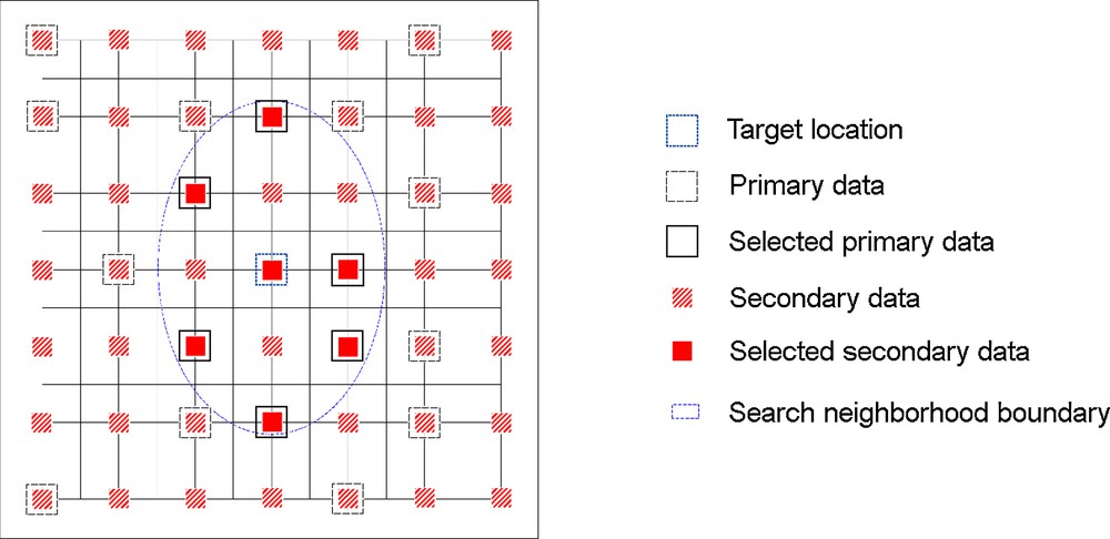
(Color online.) Data selection for collocated cokriging (case of two variables, in which it is of interest to simulate the primary variable at the target location).
2.2 Turning bands cosimulation
2.2.1 Factorizing the target vector random field
To jointly simulate the components of Y, one can split this vector random field as follows:
| (3) |
In accordance with the linear coregionalization model, Y1,…, Ys are independent vector Gaussian random fields, with B1ρ1,…, Bsρs as their respective matrices of direct and cross covariance functions. Since each coregionalization matrix is positive semi-definite, it can be decomposed as follows:
| (4) |
Let Ws be a vector random field with independent components, each with covariance function ρs. Then, it can be shown (Emery, 2008b) that the random field As Ws has the same correlation structure as Ys. The simulation of the target vector random field Y therefore boils down to simulating independent scalar random fields (the components of Ws for s = 1,…, S) with covariance functions equal to the basic nested structures used in the linear coregionalization model.
2.2.2 Turning bands univariate simulation
The simulation of the components of Ws can be performed via any multivariate Gaussian simulation algorithm. In the present case, the turning bands algorithm is chosen for its accuracy and computational efficiency. In a nutshell, this algorithm consists in drawing many lines in space, with random or, preferably, quasi-regular orientations, and simulating a one-dimensional random field along each line (Lantuéjoul, 1994, 2002). By adequately choosing the covariance function of such one-dimensional random fields, their superposition provides a multi-dimensional random field with the target covariance function, the distribution of which is practically Gaussian by virtue of the central limit theorem. The application of the method is therefore controlled by the number of lines used and by the way to simulate the basic one-dimensional random fields. The reader is referred to Emery and Lantuéjoul (2006) for mathematical details on these aspects.
2.2.3 Conditioning to data
In order to make the simulated vector random field conditional to a set of pre-existing data, one can post-process the realizations obtained by turning bands (non-conditional simulation) in order to turn them conditional. This step is based on cokriging the difference between the simulation at the data locations and the actual conditioning data values (Chilès and Delfiner, 2012; Emery, 2008b; Journel and Huijbregts, 1978). Note that cokriging can be performed even when the random fields to be simulated are not observed at the same locations (Wackernagel, 2003), so that the conditioning process does not lose information whatever the design of the conditioning dataset, either isotopic or heterotopic.
3 Synthetic analysis
One approach to assess the quality of a simulation algorithm is to compare the experimental statistics of a set of realizations (e.g., the mean value or the variogram calculated for given lag separation distances) with the underlying model statistics (Leuangthong et al., 2004). However because the realizations are constructed over a bounded domain D (represented by a finite set of spatial locations), some deviations or “fluctuations” between experimental and model statistics are expected, even if the simulation algorithm is exact. In this context, statistical testing can be used to reach a solid conclusion on whether or not the realization statistics agree with the model statistics (i.e., whether or not the fluctuations are within acceptable limits). In particular, one can check the reproduction of the mean value and of the variogram at specific lag distances (Emery, 2008a).
The synthetic case study shown in this section consists in simulating a single Gaussian random field with zero mean and isotropic spherical variogram on a two-dimensional regular grid D with 100 × 100 nodes. Two cases are considered: in the first one, the variogram has a range of 15 units and no nugget effect, while in the second case the variogram has a range of 60 units and 30% relative nugget effect. Both the turning bands and the sequential Gaussian algorithms are used to produce N = 100 independent non-conditional realizations, using publicly available codes (Deutsch and Journel, 1998; Emery and Lantuéjoul, 2006). For sequential simulation, a moving neighborhood containing up to 64 previously simulated points (8 per octant) and a multiple-grid strategy with three nested grids are considered, whereas for turning bands, one thousand lines are used for simulation. The other parameters (variogram model, number of realizations and output grid) are the same for both the sequential and turning bands algorithms.
3.1 Testing the reproduction of the mean value
Consider the average of the Gaussian random field over the whole grid:
| (5) |
| (6) |
Student test on the mean for synthetic non-conditional simulations.
| Simulation algorithm | Variogram range | Absolute value of T statistics |
| Turning bands | 15 | 0.9617 |
| 60 | 0.92259 | |
| Sequential simulation | 15 | 0.17286 |
| 60 | 0.64154 |
3.2 Testing the reproduction of the variogram
Fig. 2 compares the experimental variograms of the realizations with the underlying variogram model. It is seen that, on average over the realizations, the variogram is well reproduced with the turning bands method, whereas a bias is perceptible for the sequential algorithm, with an exaggerated range for the variograms of the realizations and a different behavior at short distances in the case of the model with nugget effect. This visual appraisal can be confirmed by statistical testing.
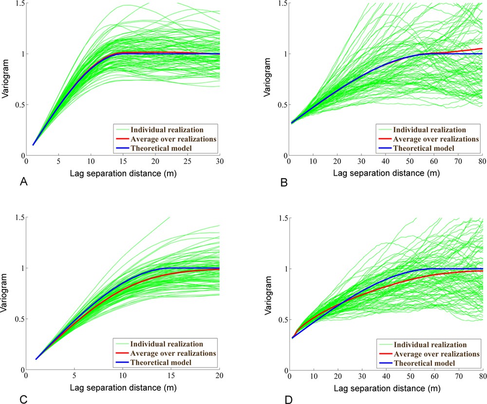
(Color online.) Variogram reproduction for spherical variogram of range 15 and no nugget effect (left) and spherical variogram of range 60 and 30% relative nugget effect (right). A, B. Turning bands. C, D. Sequential simulation.
For a given lag separation vector h, let us denote by Γ(h) the experimental variogram of the simulated random field and by γ(h) the theoretical variogram model. Let and S2(h) be the sample mean and sample variance of Γ(h), calculated over N independent realizations. For sufficiently high N, both and S2(h) are approximately normally distributed (due to the central limit theorem) and independent, so that one should have (Emery, 2008a):
| (7) |
As for the case of the mean value, if the absolute value of the left-hand side member is greater than a critical value (for a pre-specified significance level), one will reject the null hypothesis that the variogram of the simulated field at lag h is equal to γ(h). Otherwise, the null hypothesis is accepted and the simulation algorithm is validated in what refers to variogram reproduction. The test has been performed on the realizations obtained by turning bands and sequential simulation for five lags (10, 20, 30, 40 and 50) and a significance level of 0.05. The results (Table 2) do not present any case of rejection for turning bands simulation, indicating that the variogram is indeed accurately reproduced, whereas sequential simulation has a rejection rate of 50%.
Student test on variogram for synthetic non-conditional simulations.
| Simulation algorithm | Variogram range | Absolute value of T-statistics | ||||
| Lag 10 | Lag 20 | Lag 30 | Lag 40 | Lag 50 | ||
| Turning bands | 15 | 0.47958 | 0.13415 | 0.10243 | 1.1527 | 0.8572 |
| 60 | 0.13575 | 0.37503 | 0.2262 | 0.11128 | 0.3551 | |
| Sequential simulation | 15 | 7.5313 | 1.0281 | 0.68336 | 0.69996 | 1.4693 |
| 60 | 14.5126 | 0.79557 | 2.6556 | 3.4024 | 3.2084 |
The previous results concern the reproduction of the variogram at five different lags considered separately. One can also test for the reproduction at the same five lags simultaneously, by using a Hotelling test that can be seen as a multivariate extension of the Student test (Emery, 2008a). The results (Table 3) confirm the accuracy of variogram reproduction for turning bands simulation and the bias for sequential simulation.
Hotelling test on variogram for synthetic non-conditional simulations.
| Simulation algorithm | Variogram range | Hotelling statistics |
| Turning bands | 15 | 3.0394 |
| 60 | 4.3194 | |
| Sequential simulation | 15 | 120.2051 |
| 60 | 815.0394 |
Although limited to a single variable, these experiments demonstrate that the choice of the simulation algorithm has an impact on the quality of the results. In particular, beyond the visual inspection of the variograms of realizations, the Student and Hotelling tests prove that there is statistical evidence that sequential Gaussian simulation fails in reproducing the target spatial correlation structure (variogram), whereas turning bands proves to be accurate. The problem of sequential simulation stems from the iterative nature of the algorithm: the error made at each stage by using a moving neighborhood approximation propagates at the next stages, insofar as the value simulated at one location is used as a conditioning data for all subsequent locations (Emery and Peláez, 2011). Let us now examine what happens in a multivariate case, through a case study on real data.
4 Case study: Dar-Alu porphyry copper deposit
4.1 Data presentation
The Dar-Alu copper deposit is located at 29°24’46.6“N and 57°05’56.9”E, at about 135 km away from Kerman city, southeastern Iran. It is situated in the Urumieh–Dokhtar magmatic arc belt (Shafiei and Shahabpour, 2008) and consists of rhyodacite porphyry, silicified granodiorite porphyry, microgranodiorite, tonalite and rhyolithe rocks. The classical alteration for copper ore deposits, such as sericitization and chloritization, prevails in the area and the mineralization mainly consists of pyrite, chalcopyrite, sphalerite, bornite, covelite, chalcocite, magnetite, hematite and limonite, distributed in oxide, leach, supergene and hypogene zones (Salehian and Ghaderi, 2010).
A data set has been obtained from an exploration drilling campaign, where sample cores from 69 drill holes were analyzed for Cu (%), Mo (ppm), Ag (ppm), Pb (ppm), and Zn (ppm). For statistical analyses, the data have been composited at a regular length of two meters. The main statistics and experimental distributions of the analyzed grades are presented in Table 4.
Basic statistics of grade data (Dar-Alu deposit).
| Variable | Mean | Standard deviation | Minimum | Lower quartile | Median | Upper quartile | Maximum |
| Cu (%) | 0.24 | 0.22 | 0.00 | 0.06 | 0.19 | 0.35 | 3.32 |
| Mo (ppm) | 48.18 | 83.00 | 0.00 | 11.61 | 29.31 | 58.18 | 3686.52 |
| Ag (ppm) | 0.56 | 0.63 | 0.00 | 0.18 | 0.41 | 0.75 | 22.73 |
| Pb (ppm) | 16.70 | 106.00 | 0.00 | 6.00 | 9.87 | 17.00 | 8564.29 |
| Zn (ppm) | 76.35 | 115.03 | 0.00 | 41.26 | 63.56 | 92.09 | 8016.48 |
4.2 Geostatistical modeling
The modeling stage consists of the following steps:
- • in order to have representative distributions of the original grade data, cell declustering is performed to correct for the irregular sampling design (Pyrcz et al., 2006);
- • each grade variable is transformed into a standard Gaussian variable (Deutsch and Journel, 1998). The different Gaussian variables appear to be cross-correlated (Table 5), especially between copper and molybdenum and between lead and zinc. These correlations can be explained because of similar geochemical and paragenetic properties in arc-related copper molybdenum deposits (Taylor et al., 2012);
- • the marginal binormality of the pairs of transformed variables is validated by examining their scatter diagrams, which exhibit an elliptic shape (Fig. 3). In turn, the spatial binormality of the transformed variables is validated by checking that their experimental madograms are approximately proportional to the square roots of their experimental variograms (Fig. 4) (Emery, 2005);
- • variogram analysis is performed on the transformed data in order to model their joint correlation structure. Since no obvious anisotropy was detected, omnidirectional sample variograms were calculated and fitted with isotropic models, using mixtures of six basic nested structures: a nugget effect and isotropic spherical models with ranges 30 m, 100 m, 150 m, 300 m, and 600 m, respectively. The fitting of the coregionalization matrices was achieved by recourse to a semi-automated fitting algorithm (Emery, 2010; Goulard and Voltz, 1992). The results of the fitting are partially displayed in Fig. 5. Positive semi-definiteness of the coregionalization matrices (each of size 5 × 5) is imposed by the fitting algorithm, which ensures the validity of the coregionalization model.
Experimental correlation matrix for transformed (Gaussian) variables (Dar-Alu deposit).
| Cu | Mo | Ag | Pb | Zn | |
| Cu | 1 | ||||
| Mo | 0.69 | 1 | |||
| Ag | 0.42 | 0.31 | 1 | ||
| Pb | 0.10 | 0.03 | −0.17 | 1 | |
| Zn | 0.33 | 0.05 | 0.12 | 0.43 | 1 |
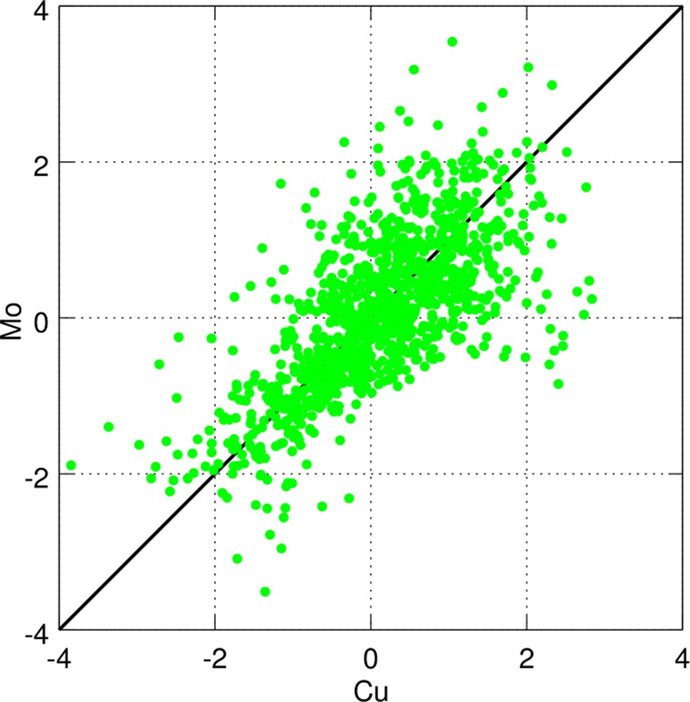
(Color online.) An example of scatter plot between Gaussian variables (Cu vs. Mo).
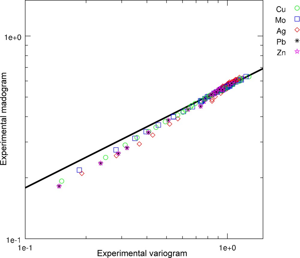
(Color online.) Experimental madograms of the Gaussian variables as a function of their experimental variograms. In case of bivariate normality, the points should be distributed along the thick solid line.
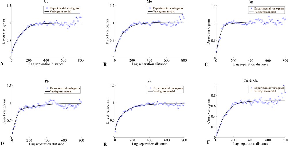
(Color online.) Sample (crosses) and modeled (solid lines) direct and cross variograms of Gaussian variables. For brevity, only the Cu–Mo cross-variogram is displayed, which corresponds to the pair of variables with the highest cross-correlation, although the fitting has been achieved with all the cross-variograms.
4.3 Joint simulation of grades
Cosimulation is performed on a regular grid with a mesh of 10 m × 10 m × 12 m. In both algorithms (sequential and turning bands), simple cokriging is used with a moving neighborhood of horizontal radius 500 m and vertical radius 250 m, containing up to eight original data points in each octant and, for sequential simulation, up to eight previously simulated points in each octant, in addition to the original data (one may therefore have up to 64 selected points for turning bands and up to 128 selected points for sequential simulation, each point consisting of a vector with five components). Furthermore, the same conditioning data set (original drill hole data), Gaussian transformation functions, direct and cross variogram models and numbers of realizations (100) are considered for both algorithms. Two variants are tested for sequential simulation: full cokriging and collocated cokriging, as explained in Section 2, in both cases using a multiple-grid strategy with three nested grids. For turning bands, one thousand lines are used, as in the synthetic case study.
In order to validate the results, the distributions of the simulated grades are compared with the distributions of original data, through quantile-quantile plots. It is expected that, on average over many realizations, the plots fit the diagonal lines, indicating an accurate reproduction of the data distributions. This is what effectively happens for the realizations obtained with both turning bands and sequential simulation (Fig. 6).
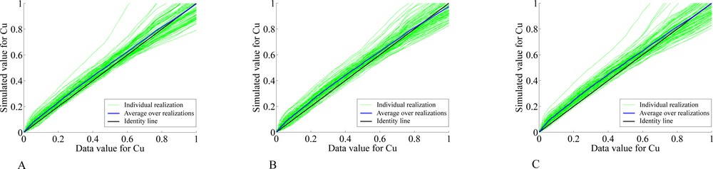
(Color online.) Quantile–quantile plots between original copper grades and simulated copper grades, for turning bands cosimulation (A), sequential cosimulation with full cokriging (B) and sequential cosimulation with collocated cokriging (C).
To check that the realizations also reproduce the dependence relationships between grades, one can calculate the correlation coefficients between the Gaussian transforms of simulated grades in each realization. It is expected that these coefficients fluctuate around the experimental correlations (Table 5), for instance, 0.69 for Cu-Mo. This situation happens for turning bands and sequential cosimulation with full cokriging, but not for sequential cosimulation with collocated cokriging (Fig. 7). In the latter case, the correlations reproduced by the realizations are, on average, lower than the expected correlations. This bias can be explained because, in comparison with full cokriging, collocated cokriging is likely to discard many data of the covariates (Fig. 1), which entails a poor reproduction of the dependence between the variables to be simulated (proof in Appendix, supplementary data).
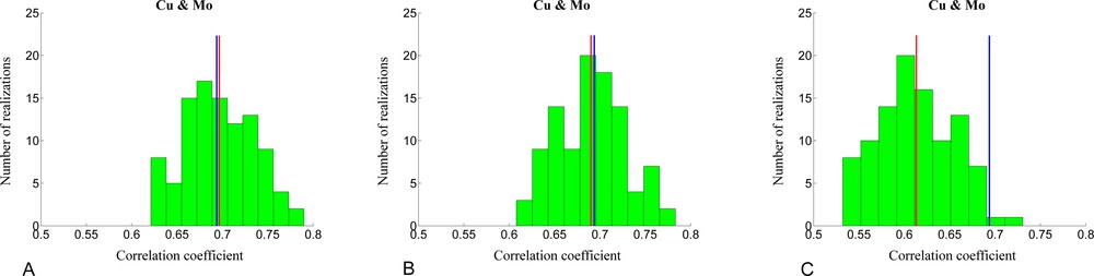
(Color online.) Correlation coefficients between Gaussian random fields simulated with turning bands (A), sequential cosimulation with full cokriging (B) and sequential cosimulation with collocated cokriging (C). For brevity, only the correlation between copper and molybdenum is displayed. The average correlation is represented with a red line, while the true data correlation is represented with a blue line.
Another criterion for assessing the quality of each simulation algorithm is to check the reproduction of the direct and cross variograms of the simulated Gaussian random fields. The results indicate that the direct variograms are well reproduced by all the algorithms (Fig. 8) and the cross variograms are well reproduced with turning bands and, to a lesser extent, with sequential simulation using full cokriging. In contrast, sequential simulation using collocated cokriging leads to an inaccurate reproduction of the cross variograms (Fig. 9), which can be explained because, unless for very specific coregionalization models, such a cokriging is usually a poor approximation of full cokriging (Chilès and Delfiner, 2012; Rivoirard, 2001, 2004). To improve the reproduction of the cross variograms with sequential simulation, an alternative would be to follow the same workflow as for turning bands (Section 2.2), i.e. to (i) factorize the target vector random field, (ii) sequentially simulate the factors, (iii) recombine the simulated factors and finally (iv) condition to the original data by cokriging. This would avoid using cokriging in the sequential simulation stage, insofar as the factors would be simulated separately at step (ii), so that the errors due to a moving neighborhood implementation would not propagate from one factor to another one. Provided that the spatial correlation of the factors is accurately reproduced, so will be the direct and cross variograms of the target vector Gaussian random field.
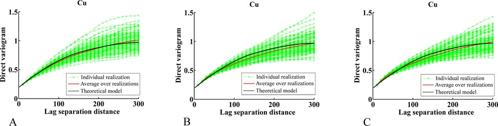
(Color online.) Direct variograms of Gaussian random fields simulated with turning bands (A), sequential cosimulation with full cokriging (B) and sequential cosimulation with collocated cokriging (C). For brevity, only the variograms for copper are displayed.
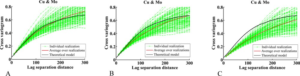
(Color online.) Cross variograms of Gaussian random fields simulated with turning bands (A), sequential cosimulation with full cokriging (B) and sequential cosimulation with collocated cokriging (C). For brevity, only the cross variograms between copper and molybdenum are displayed.
4.4 Cross validation
The previous analyses allowed assessing the quality of the simulation algorithm (turning bands or sequential) but do not provide much insight into the chosen stochastic model (namely, a Gaussian random field model with the spatial correlation structure given by the variograms fitted in Fig. 5). To corroborate the suitability of this model to the data, a leave-one-our cross-validation exercise is proposed, which consists in cosimulating the grades at each data location, conditionally to the information available at the other locations only, then in comparing the actual data grades with the average of the simulated values (considered as the best prediction of the true grades) at the data locations. For the sake of simplicity, the turning bands algorithm is used for cosimulation.
It is seen (Fig. 10) that, for each element, the average of simulated grades fluctuates around the true data grade and that the conditional regression between true and simulated grades is close to the identity, which reflects conditional unbiasedness (Rivoirard, 1987; Vann et al., 2003). These results indicate that the Gaussian model used to represent the grade data is adequate in this case study, as the results of simulation are in agreement with the actually observed data.
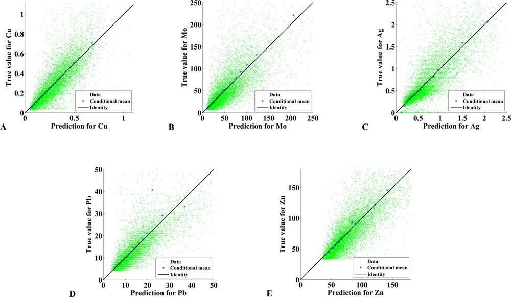
(Color online.) Scatter plot between true data grades (ordinate) and predicted grades (abscissa) for (A) copper, (B) molybdenum, (C) silver, (D) lead and (E) zinc. Predicted grades are calculated as the average of 100 realizations obtained with turning bands.
5 Conclusions
This study aimed at assessing the performance of two popular algorithms (turning bands and sequential) for jointly simulating coregionalized variables, through a synthetic case study (univariate) and a real case study (multivariate) from a multi-element deposit. The algorithms are fed with the same inputs: original conditioning data and Gaussian transformation functions in the real case study, variogram models, moving neighborhoods, output grids and numbers of realizations. The only differences are the use of previously simulated points in sequential simulation and the use of a finite number of lines in turning bands simulation, which is explained by the specificities of each algorithm.
In both cases, turning bands accurately reproduces the spatial correlation structure, measured by the direct and cross variograms of the coregionalized variables under consideration, while sequential simulation produces some biases. Such biases are explained by a propagation of errors caused by the use of a moving neighborhood to determine the successive conditional distributions. This problem is more severe in the multivariate case when using collocated cokriging, in which case the reproduction of the cross variograms turns out to be poor. Accordingly, the choice of the simulation algorithm is relevant to accurately reproduce regionalized properties and the turning bands algorithm appears as an alternative of the sequential algorithm for the modeling of multi-element deposits.
Acknowledgements
The authors thank the reviewers, Dr. Denis Marcotte and Dr. Joao Felipe Costa, for their recommendations that helped to improve the paper, and to Mr. Esfahanipour R. from the National Iranian Copper Industry Co. (NICICO) for granting access to the Dar-Alu copper deposit exploration data. The last two authors also acknowledge the funding by the Chilean Commission for Scientific and Technological Research, through Project Conicyt/Fondecyt/Regular/No. 1130085.