

1 Introduction
Geological and geophysical observations and measurements provide limited information on the 3-D structure and notably on the formation and evolution of faults, particularly at large scale. Natural fault structure is far from simplistic planar or single-surface schemes and has a complex 3-D architecture with different segments and branches that can be reactivated at different periods of the fault's evolution. Microseismicity data indicates that the material around the faults undergoes damage during the interseismic periods at a distance up to ± 10–30 km from the fault. In some areas, this damage (microseismicity) is diffused (during the observation time), but in others, it is concentrated in narrow zones corresponding probably to fault branches (e.g., Bulut et al., 2012; Valoroso et al., 2014). Co-seismic ruptures (e.g., Fu et al., 2005), the distribution of aftershocks (e.g., Fukuyama et al., 2003) as well as the surface traces of fault branches and segments (Perrin et al., this issue) also reveal a complex structure of natural faults. The fault branches and segments themselves are not zero-thickness interfaces but represent zones of various thicknesses where the material undergoes continuous damage and property changes (e.g., Caine et al., 1996; Faulkner et al., 2010; Haines et al., 2013; Schulz and Evans, 1998). Understanding all these processes via the development of progressively more adequate mechanical models based on both physical analysis and geological data, is a necessary step toward a possibility of earthquake prediction. Knowledge of the structure of natural faults at different scales and the associated variations of stress and porosity also is fundamental for various applications in oil industry, waste storage, or hydrothermal energy.
The mechanical (experimental/physical or numerical) models can partially fill the gap between the complexity of natural faults and the fragmentary information we have about them. Of course, the models are always simpler than nature, but they must be sufficiently realistic to capture essential features of the natural process. Most of existing models are purely elastic and therefore do not meet the above requirement. The material damage, fracturing, and faulting are essentially non-elastic phenomena caused by strongly non-linear and irreversible deformation. A description of these processes requires constitutive models that become more sophisticated with the progress in our understanding of the rock behavior, which is attested by the extensive literature on this subject (D’Adetta and Ramm, 2005; Kamrin et al., 2007; Lyakhovsky and Ben-Zion, 2014; Mas and Chemenda, 2015; Nicot and Darve, 2007; Nova et al., 2003; Sulem et al., 1999; Tengattini et al., 2014; Wong and Baud, 2012; Zhu et al., 2010) to mention only a few papers. Recent processing of large data sets from mechanical tests of different rocks (Mas and Chemenda, 2015) shows, for example, that all constitutive properties (such as the internal friction, dilatancy, and cohesion) change with deformation, meaning that at each stage of inelastic straining the material is different. This is in agreement with the previous studies (e.g., Sulem et al., 1999) on initially intact rocks but also on severely strained gouge rocks that undergo microstructure and property change during deformation (e.g., Haines et al., 2013), which must be taken into account in the models of faulting.
As a first step, a simplified version of the constitutive model from (Mas and Chemenda, 2015) is used in this paper, but a more general formulation is presented as well. This model is applied to simulate numerically the formation of a strike-slip fault (fault zone/system) under Riedel-type loading conditions. Unlike Riedel experiments, both analog (e.g., Bokun, 2009; Dooley and Schreurs, 2012; Naylor et al., 1986; Richard et al., 1995; Riedel, 1929; Tchalenko, 1970) and numerical (Braun, 1994; Stefanov et al., 2013), we apply ‘softer’ boundary conditions to the bottom of the model by imposing tractions instead of velocities, which appears to be more realistic in many geological contexts. The obtained results show a scenario of fault formation from initial distributed material damage to deformation localization resulting in Riedel shears evolving into complex 3-D fault architecture within an initially homogeneous layer. Such a scenario was obtained in a numerical model for the first time and corresponds fairly well to the initial stages of the evolution of sandbox models (e.g., Naylor et al., 1986).
2 Setup and constitutive model
2.1 Modeling Setup
The model represents a layer (Fig. 1a) with elastoplastic properties described in the next section. The layer is subjected to a gravity force that generates the initial stresses, characterized by the vertical gradient defined by the model density ρ and the depth as well as the acceleration due to gravity g. Along the y-parallel vertical boundaries, roller conditions (free along–boundary slip) are applied. Along the y-normal boundaries, a kinematic condition is imposed: at all corresponding points (having the same coordinates x and z) (x, 0, z) and (x, D, z) at these boundaries, the velocities are the same and equal to the velocities at points (x, D/2, z), where D is the model length in the y-direction. This annuls the boundary effects as if the model were infinite in the y-direction. A shear stress, τzy, which increases progressively during deformation, is applied to the layer bottom, which is fixed in the z-direction. The x-profile of this stress is shown in Fig. 1b and does not vary along y. The resulting y-displacement (uy) profile is presented in Fig. 1c. It shows a smooth change in the displacement (and hence of the velocity) in the x-direction. In the classical Riedel experiment, the deforming layer is supposed to be coupled to the two adjoining rigid basement boards displaced horizontally one past the other. Therefore the x-profile of uy seems to be imposed to have a shape similar to that of τzy in Fig. 1b. One can consider that, in our numerical experiments, there is a relatively weak plastic layer between the deforming model and the rigid boards. This layer transmits tractions (rather than velocities) to the model base. The velocities and displacements are not imposed and can vary both in time and space during the experiment. This setup also can correspond to the constant friction condition at the interface between the layer and the rigid boards and seems to be more realistic in many geological situations, as, for example, at the crustal scale, when a quasi-brittle upper crust is underlined by a weak and ductile lower crust. The magnitude of the applied traction τzy is increased during cycling progressively and slowly enough to keep the process quasi-static.
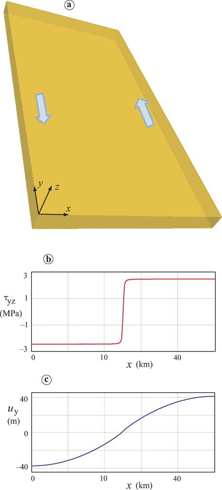
(Color online.) Modeling setup, showing elastoplastic model layer (a) and a profile of shear stress τzy (b) applied to the layer bottom in the y-direction. Also is shown a profile of the displacement uy (c) in the same direction at the model bottom for a certain stage of the elastic loading. The model sizes in the x, y, and z directions are respectively: L = 50 km, D = 100 km, H = 5 km. The reference model parameter values are: Young's modulus E = 1 × 10¹⁰ Pa; Poisson's ratio v = 0.25; internal friction coefficient α = 0.6; dilatancy factor β = 0.1; initial and end normalized hardening moduli, hini = 0.001 and hend = −0.12 (the latter is reached when ); initial and residual cohesion, kini = 1 × 10⁷ Pa and kend = 2 × 10⁵ Pa; density ρ = 2700 N/m3. The cubic grid size is 320 × 640 × 32.
2.2 Constitutive model
To describe the inelastic behavior, we use two invariant yield F(σij) and plastic potential G(σij) functions
| (1) |
| (2) |
According to the experimental data (e.g., Mas and Chemenda, 2015), the normalized hardening modulus h progressively reduces during the material loading. This modulus is defined as , where G is the shear modulus. For the presented constitutive framework, (Chemenda, 2007). We assume a linear function
| (3) |
The elastic properties of the model both before and after reaching the yield condition are described by Hook's equations with Poisson's ratio v = 0.25 and Young's modulus E that was varied from 1 × 10¹⁰ Pa to 8 × 10¹⁰ Pa, corresponding respectively to the sedimentary and crustal rocks. The modeling results do not depend much on this modulus. Therefore, we present results obtained only with one value, E = 1 × 10¹⁰ Pa.
The formulated constitutive model has been implemented into the finite-difference 3-D dynamic time-matching explicit code Flac3D (Itasca, 2012) used for the numerical modeling in this work. The simulations were carried out in large-strain mode, with different model parameters. Below we report the results from the representative (reference) model (the model parameter values are given in the caption of Fig. 1) and present another model with more ductile behavior.
3 Results
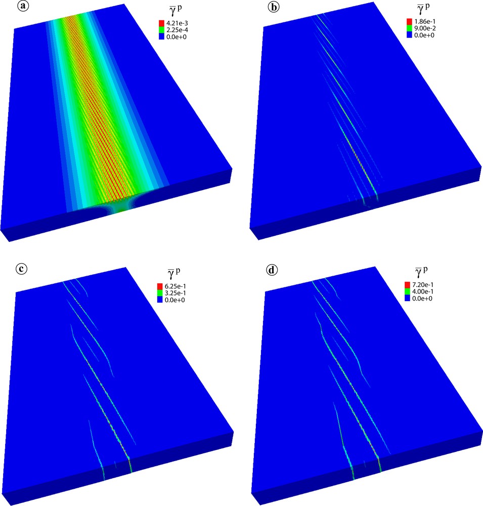
During the initial stages of the model's evolution (caused by the increasing traction at the layer's bottom), its response is purely elastic. At a certain stage, the inelastic deformation starts at the surface in the axial (along y) area (Fig. 2a). The inelastic zone thickens and rapidly widens in the x-direction (Fig. 2b). At a certain stage, the damage (inelastic deformation) starts at the model bottom (Fig. 2b). At the next stage, a dense set of parallel deformation localization bands (incipient faults) is formed. The whole band set first evolves uniformly (the inelastic deformation within all bands increases), and then one observes a sort of “band selection” process: most of the bands die, while the others continue evolving (Fig. 2c and d). The shape of uy (and y-velocity) profiles also changes during the evolution of this non-linear inelastic deformation (Fig. 3). Finally, only 4–5 well-developed bands (faults–Riedel shears) persist (Fig. 2d). They propagate first in-plane, then out-of-plane (forming splay faults according to the terminology of Naylor et al. (1986)) and new faults form as well (Fig. 2e and f). The less developed bands formed at the previous stages are not seen in Fig. 2d–f because the damage intensity (i.e., inelastic strain ) within them is much smaller than in the visible bands. The fault pattern considerably changes with depth (Fig. 4). This figure (as well as Fig. 2c) shows that the initial Riedel shears affect the model only to a depth shallower than ∼ 0.3H and that the fault branches have different dip. From Fig. 5, it can be inferred that these are normal (normal-shear) faults whose activity results in the formation of ∼ 100-m-deep valleys.
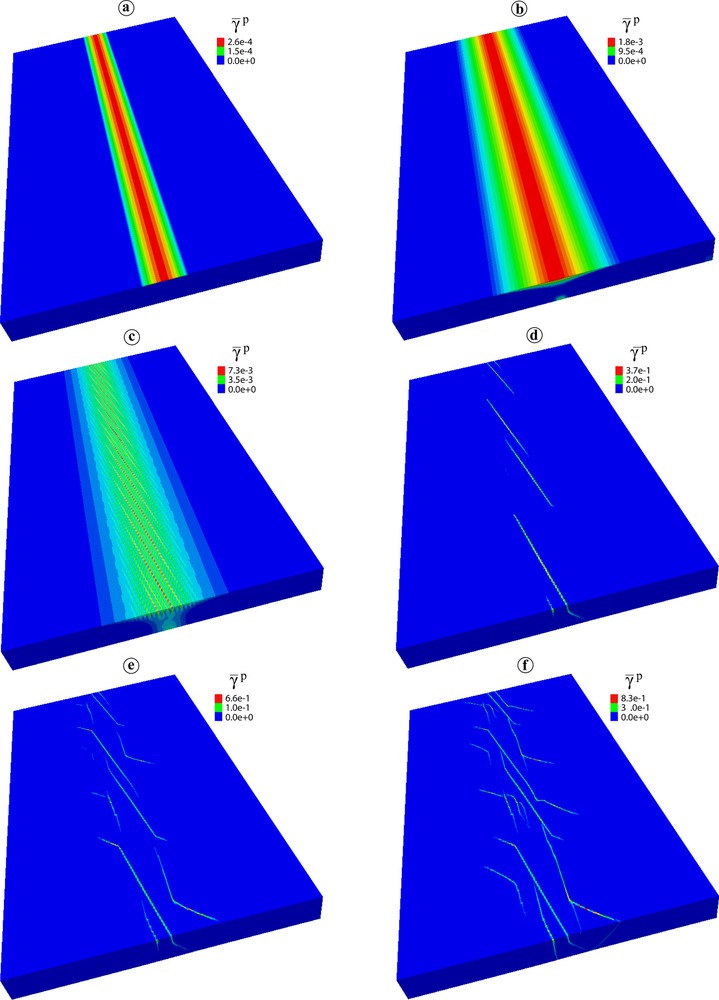
(Color online.) Evolution of the field in the reference model. The total shear displacement in (f) is 250 m.
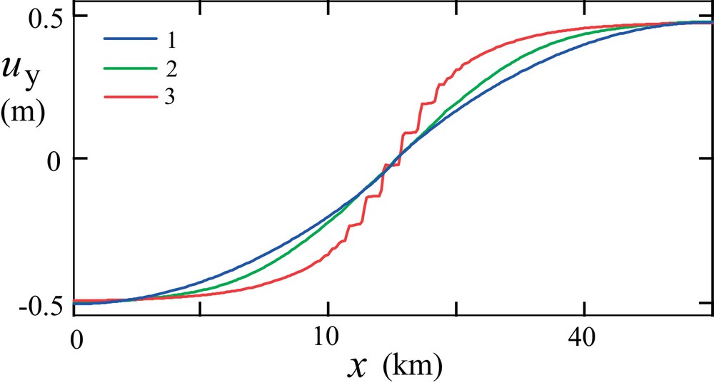
(Color online.) Along-x-axis profiles of the incremental displacement uy in the y-direction at different stages of the model's evolution (in all cases the displacement at x = 0 and x = L is ± 0.5. 1: Purely elastic deformation stage; 2 and 3: successive stages with inelastic deformation).
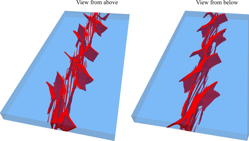
(Color online.) 3-D architecture of the fault system (shown in red are zones with ).
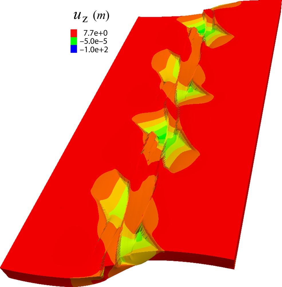
(Color online.) Vertical displacement, uz, field at the last stage in Fig. 2 showing four valleys. The model deformation is magnified by a factor of 50 to clearly display the deformation features. The indicated uz values are not affected by this magnification.
At the last stage of the model's evolution (Fig. 2f), the most active are the three fault segments (Fig. 6), but the damage affects other segments and zones as well (Fig. 7). The velocity field at the model surface, resulting from both sliding along the active at this stage fault segments and the distributed deformation, shows two counterclockwise rotating zones (Fig. 8).
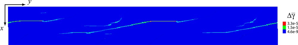
(Color online.) Incremental total (elastic and inelastic) equivalent shear strain during one calculation step (corresponds to the strain rate) at the last stage in Fig. 2.
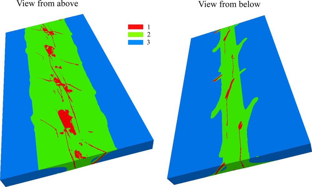
(Color online.) Mechanical state of the model at the last stage in Fig. 2. 1: zones affected by the inelastic straining in the past and active at the deformation stage shown. 2: all zones affected by inelastic straining in the past (inactive now). 3: zones that were not strained beyond the elastic limit.
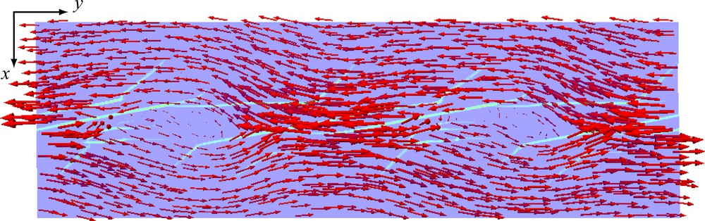
(Color online.) Velocities at the model surface on a background of the field at the last stage in Fig. 2 (only the central part of the model with faults is shown).
In Fig. 9, we present the model with the two times larger end hardening modulus, hend = −0.06. The initial stages of deformation (not shown) in this model are similar to those in the reference one.
(Color online.) Four stages of evolution of the model that differs from the reference model by 2 times higher hend: hend = −0.06. The previous evolutionary stages are similar to those in Fig. 2.
4 Concluding discussion
The modeling setup and the constitutive framework used in this work were chosen to be as simple as possible, but at the same time reproducing the principal features of faulting in the experimental sandbox models. The formation of classical Riedel shears followed by splay faulting in sandbox experiments (Naylor et al., 1986) were obtained in the numerical models presented for the first time. There are many examples of natural Riedel-type fault systems at different scales (they are given in most of the numerous papers on analogue modeling of Riedel faulting, some of which are cited in the introduction). The surface traces of the San Andreas Fault and its branches show that this large-scale fault system belongs to the same Riedel-type class (e.g., Supplementary material in Perrin et al., this issue).
Analogue and numerical models are complementary. An important advantage of numerical models is that they allow one to follow the evolution of deformation, velocity, and stress fields with great precision and in 3-D, and thus to see details hardly detectable in the experimental models. It was unexpected, for example, that inelastic deformation and fracturing/faulting start at the surface (Fig. 2a and c), but this has a simple explanation. The material strength increases with depth due to the frictional component of the strength, which grows with lithostatic pressure (or more exactly with σm). The strength therefore is the lowest in upper horizons where fracturing occurs first under the conditions tested.
The inelastic deformation strongly reduces the tangent modulus (the apparent stiffness), making the material's response much more compliant. On the scale of the modeled layer, the compliance of the response increases with the increase in the material volume involved into the inelastic deformation and with the reduction of the hardening modulus. That is why the gradient of the incremental displacement uy (or of the displacement rate ) across the fault zone increases with inelastic deformation and with the material volume involved into this deformation (Figs. 2a–c and 3). The profiles like those in Fig. 3 are typically obtained across the active faults during interseismic phases from GPS and InSAR data (e.g., Wright et al., 2001). Purely elastic models are usually used to interpret these profiles. Two blocks separated by a dislocation represent the crust in these models. The dislocation is locked from the surface down to a certain depth (the locking depth) and is unlocked below this depth where the blocks are allowed to move freely one past the other (Savage and Burford, 1973). By adjusting the locking depth and the spatial distribution of the elastic stiffness, one can obtain a good fit between the model and the data (e.g., Fialko, 2006). Such an approach, however, does not really contribute to the understanding of the underlying deformation mechanisms and is not satisfactory from a physical point of view. Indeed, the interseismic microseimicity clearly attests to irreversible, dissipative deformation processes affecting large areas/volumes of the crust (e.g., Bulut et al., 2012). These processes cannot be captured by elastic models. For high across-fault displacement rate gradients measured, these models require very small locking depths (a few kilometers) (e.g., Cavalié et al., 2008), which is not realistic. To avoid this inconsistency, an aseismic slip in the seimogenic zone is postulated (e.g., Jolivet et al., 2012), but a more physically sound solution should take into account the inelastic deformation in a wide fault zone, as shown in Figs. 2a–c, 4 and 7. This deformation causes an increase in the displacement gradient (Fig. 3).
In our models, the inelastic deformation starts after reaching certain (sufficiently high) stressing level proportional to the interseismic displacement, which itself is proportional to the time span from the last earthquake. A prediction from the presented models would be therefore that the across-fault displacement gradient should increase with time while approaching the next large seismic event. Although it appears to be too simplistic, this prediction seems to work, at least in some cases. The North and East Anatolian faults (NAF and EAF, respectively) are good examples confirming this prediction (Cavalié and Jonsson, 2014). For the NAF, at the location where the last ruptures occurred in 1949 and 1992, the across-fault displacement rate gradient is relatively low and corresponds to a locking depth of 14 km. For the EAF, where the last rupture occurred in the 19th century, this gradient is much higher, with the predicted (from the elastic model) locking depth of only 3 km. Similar results were obtained for the Haiyuan fault, where high gradients were measured along a segment that did not rupture since 1092 AD. The adjacent segment that ruptured in 1920 shows a much lower gradient (Cavalié et al., 2008; Jolivet et al., 2012).
The reported numerical models show that the first generation of a dense set of Riedel shears does not exceed in depth ∼ 1/3 of the model thickness H (∼ 1.5 km); they are the deepest along the model axis (Fig. 2c). Only a few faults of this set persist with further evolution. They cut through the whole model thickness, undergo some in-plane propagation, and then rapidly change their orientation (Fig. 2e). New fault segments are formed as well. At the model's base, the faults are not aligned along the y-axis (Fig. 4) as they would be in classical Riedel experiments, but have a freedom to deviate from this axis because the model bottom is not kinematically constrained (as described in section 2.1).
Fig. 7 shows that the width of the damage zone at the surface is ∼ 5H (25 km for H = 5 km in the presented model), while at the bottom, it is only ∼ 2H (excluding fault branches). This zone therefore has a flower-type structure, which also characterizes natural strike-slip faults (e.g., Sylvester, 1988). Such structures (but not Riedel shears) have been obtained in numerical models by Finzi et al. (2009) using a different constitutive framework, but their width is much smaller than in our models, only several kilometers, which may correspond to the core (central) zone in our models with the highest damage intensity. The microseismicity however affects a zone wide of several dozen kilometers, as indicated in the introduction.
Each point of the damage zone in Fig. 7 underwent active damage at some stage of the model's evolution. At the stage shown in this figure, only some fault segments and zones are active (in red). At the next stage, other fault segments and zones will be active. Such damage events can be viewed as microseismicity within a wide fault zone, although the time-scale of the presented modeling does not allow us to talk about seismic cycles. Moreover, this modeling is not designed to be specifically applied to large-scale seismic faults. It can correspond to the faulting within a sedimentary layer having approximately the same coefficients α and β, and a comparable ratio k/ρgH. If these conditions of physical similarity are not met (for example, when k is the same, but H is much smaller–a strong, thin layer), the modeling should be done with other parameters.
The specificity of a large (crustal) scale faulting (compared to the faulting in a relatively thin layer) is that practically all material properties change with depth, which should certainly affect the results. Fig. 9 shows, for example, that the increase in the hardening modulus hend (which corresponds to a more ductile material response) leads to very different fault evolution and pattern. This suggests that the fault pattern at depth (where the material is more ductile) should be rather similar to that shown in Figs. 9 and, at a shallow depth, to the one in Fig. 2, although it is clear that faulting does not occur independently at different depths. Further modeling is needed to obtain more complete scenarios.
Acknowledgments
This work is a tribute to our friend and colleague Jean-Francois Stéphan. The paper has been reviewed by Stéphane Dominguez and Associate Editor Isabelle Manighetti.