

1 Introduction
The author Nassim Taleb published an influential book in 2007 called the “The Black Swan” with the subtitle “The impact of highly improbable events”. According to his definition, a “black swan event” is a statistically improbable event that occurs with no prior warning and has a major effect in the field in which it occurs. Though the main focus of the book is on economic events, the author notes that such events also occur in science, religion, culture and politics.
The discovery of the Antarctic Ozone Hole in the mid-1980s was surely a black swan event in environmental sciences. It was undoubtedly a total surprise. Prior to its discovery the scientific consensus was that the effect of Ozone Depleting Substances (ODS), such as chlorofluorocarbons (CFC), would be first seen near 40 km where the natural variability of ozone is relatively small. Since the ozone amount near 40 km is small, the total ozone column above the surface was expected to change very little. Globally averaged change in total column ozone was expected to be only about 1%/decade. Given the large natural variability of the total ozone, and the difficulty of maintaining long-term calibration of instruments to such high accuracy, such changes were not expected to be seen in the data for a decade or longer. Changes in the total column ozone over Antarctica turned out to be much larger and occurred over much shorter time period. So, statistically the development of the Ozone Hole was a highly improbable event.
Finally, the images of the Ozone Hole produced from satellites captured the attention of public and media all over the world, and led to scientific field campaigns using aircraft, balloon, and advanced ground-based instruments deployed over Antarctica, coupled with new laboratory measurements, to better understand the chemistry of the stratospheric ozone layer. Though, plans to phase out the ODSs had started before the discovery of the Ozone Hole, and arguably the signing of the Montreal Protocol in 1987 was not directly influenced by it, there is no doubt that the discovery of the Ozone Hole greatly influenced the public and policy makers in accepting actions recommended by the signatories of the Montreal Protocol to phase out the production of gases that provided broad societal benefits and impacted a multi-billion-dollar global chemical industry.
In his book, Dr. Taleb also discusses the chaos that occurs when black swan events occur and how misinformation and theories are created post-hoc to explain what did or did not occur. In this paper, we discuss such events surrounding the discovery of the Antarctic Ozone Hole. A previous version of this paper appeared in the Proceedings of the Symposium for the 20th Anniversary of the Montreal Protocol (Bhartia, 2009).
2 History of ozone measurement over Antarctica
Prior to the discovery of the ozone hole, the ozone layer over Antarctica had been monitored from ground-based and balloon-borne instruments for many decades, and by satellites since 1970. A Dobson spectrophotometer at NOAA's South Pole Station had measured total ozone column since 1961. The data from this station as well as from other stations around the world had been archived at the World Ozone and Ultraviolet Radiation Data Center (WOUDC), Atmospheric Environmental Service, Downsview, Canada. WOUDC used to publish these data in the so-called “Redbooks” that were distributed to institutions all around the world. WOUDC also archives and distributes ozonesonde data that provide ozone vertical profile information from the surface to about 30 km.
Routine measurement of Antarctic ozone from satellites started in 1970 with the launch of the Backscatter UV (BUV) instrument on NASA's Numbus-4 satellite. Though, in 1970, the depletion of the ozone layer was not an issue, the instrument was fortuitously designed to measure ozone density near 40 km as well as the total column ozone above Earth's surface (Mateer et al., 1971). Both these measurements subsequently became important in understanding the effect of ODSs on the ozone layer. This instrument had occasionally measured very low total ozone values over Antarctica, lower than values measured anywhere else in the world. However, at the time it was not clear whether such values were caused by measurement error or some real geophysical effect.
Though an instrument similar to BUV was flown on the Atmospheric Environment (AE) satellite in 1975, the satellite orbit confined the measurements to the tropics. A major improvement in satellite ozone measuring capability occurred with the launch of Nimbus-7 satellite in October 1978. This satellite had an infrared limb sounding instrument called LIMS to measure the ozone profile down to the tropopause but it lasted only about 7 months when the cryogen needed to cool the detectors ran out. However, the satellite also had an instrument package containing two nadir UV instruments called Solar Backscatter UltraViolet (SBUV) and Total Ozone Mapping Spectrometer (TOMS). The SBUV was an advanced version of the BUV instrument with both total ozone and profiling capability, while the TOMS was designed to be a global total ozone mapping sensor with no profiling capability. In 1976 NASA formed an Ozone Processing Team (OPT) to process the data from these instruments with a science advisory team led by Donald Heath to oversee the algorithm development efforts. Unfortunately, within a year both UV instruments suffered degradation due to contaminants deposited on the optical surfaces. An international scientific panel formed by NASA to assess the problem concluded that the degradation had made these instruments unsuitable for monitoring the relatively small changes in the ozone layer predicted by the models, both at 40 km as well as in total ozone. A solution to improve the total ozone record was found in circa 1983 and was implemented. However, given slow computers and the lack of digital data links to transport data, the data processing was running nearly 9 months behind real time though mid 1984. Therefore, the October 1983 data that played a key role in the discovery of the Ozone Hole was not processed until June 1984.
3 Discovery of the Ozone Hole
In May 1985, Farman et al. (1985) reported seeing a large secular decrease in the total ozone column over the Halley Bay station in Antarctica operated by the British Antarctic Survey. It was the first such paper published in a widely circulated peer-reviewed scientific journal and the first to suggest an explanation of why the observed decrease occurred only in September/October. They postulated that this had something to do with the very low temperatures that occur in the Antarctic polar vortex in these months. Though it turns out that previously Chubachi (1984, 1985) had reported seeing unusually low ozone values in the lower stratosphere in the balloon data taken at the Japanese Syowa station in Antarctica, these results were reported in a conference and didn’t get much notice at that time.
In August 1985, at the IAGA/IAMAP conference in Prague, Czechoslovakia Bhartia et al. (1985) showed the first map of the Antarctic Ozone Hole produced by the TOMS satellite instrument (Fig. 1). They also showed ozone profiles and seasonal cycle of total ozone produced by the companion SBUV instrument. These results confirmed the findings of Farman et al. (1985) and showed that the decrease they had observed was a continent scale phenomenon. Though this paper has not been published many of the slides were reproduced by Callis and Natarajan (1986) and some have appeared in other publications (Fig. 2).
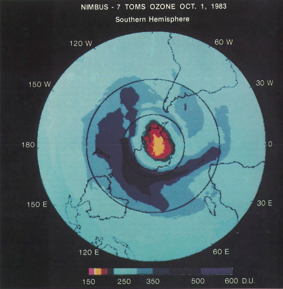
October 1, 1983 image of the Antarctic Ozone Hole shown by Bhartia et al. (1985) at the IAGA/IAMAP meeting in Prague, Czechoslovakia.

Reproduction by the Journal of Chemical Education of another vugraph presented by Bhartia et al. (1985). It shows two images of Antarctic ozone taken on the same day (October 3) but four years apart. Large decrease of total ozone over Antarctica with no discernable change in lower latitudes seen in these images contradicted the model results predicting 1%/decade decrease in global total ozone due to CFCs. Comparison with Fig. 1 shows a rotating evolving Ozone Hole that expanded in just 2 days to reach the tip of South America.
These results got lot of attention shortly thereafter in a meeting in Salzburg, Austria in late August 1985 attended by prominent scientists from around the world studying the ozone layer (Fig. 3). The meeting had been organized in 1984 by Dr. Donald Heath, the Principal Investigator of the SBUV instrument, to discuss state-of-the-art of ozone science. Prof. Sherry Rowland who later received the 1995 Nobel Prize in Chemistry, along with Prof. Mario Molina and Paul Crutzen, were also in attendance. Prof. Rowland borrowed that first Ozone Hole image from Dr. Heath and released it to New York Times, where it was published along with an article on November 7, 1985. Following that publication, many such images were published in journals and magazines all across the world. These iconic images still generate lot of attention in the public and media some 3 decades after the phenomenon was first discovered.
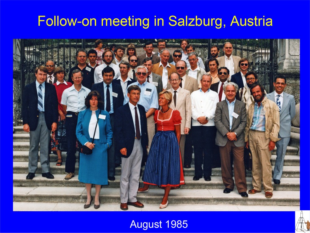
Attendees to a scientific meeting held in Salzburg, Austria in August 1985 to discuss recent developments in ozone research. The meeting was organized by Donald Health (foreground), the PI of NASA's SBUV sensor and head of the SBUV/TOMS science team. Prof. Sherry Rowland (right top corner) provided the copy of a vugraph presented at this meeting to New York Times where it was published on November 7, 1985.
4 Chaos and misinformation associated with the discovery
As Nassim Taleb discusses in his book, the discovery of the Ozone Hole also generated its share of chaos, misinformation, and missed opportunities. The first such missed opportunity occurred when Jonathan Shanklin, coauthor of Farman et al.’s (1985) paper, sent a letter to Harry Bloxom at NASA's Wallops Island Center on October 10, 1983, reporting “low ozone values of around 200 Dobson Unit” at Halley Bay and wondered if it could be “confirmed by satellite data”. He also wondered if this was “possibly connected with the El Chichon volcanic eruption” that had occurred in April 1982. In a Nov 29, 1983 reply to this letter Harvey Needleman, Head of the Balloon Projects Branch at Wallops, indicates that the letter was forward to Alfred Holland who at that time was involved in ozone measurements at Wallops. Wallops had been collecting ozone data from ground, balloons and rockets but was not directly involved with satellites. The SBUV & TOMS instruments were being managed at NASA Goddard Space Flight Center (GSFC), Greenbelt, Maryland. Though there is no record that A. Holland contacted anyone at Goddard, as we have noted before, Spring 1983 satellite data were not processed at NASA GSFC until June 1984. So, in the late 1983 no one at NASA had the results to confirm J. Shanklin's results. Moreover, since 200 DU ozone values had been seen over Antarctica in the satellite record going as far back as 1970, these low values by themselves were not surprising. What was surprising is the secular change in the Antarctic total ozone that was reported by Farman et al. some 18 months later.
A second case of missed opportunity occurred when the TOMS data processed in June 1984 revealed very low values of ozone over Antarctica in Sept/Oct 1983. Though initially it was thought that the problem was related to instrument degradation or satellite malfunction, as the satellite was well past its one year design lifetime, this was quickly ruled out. The next step, as is typical in such cases in satellite projects, was to find “ground truth” data to “validate” satellite data. The aforementioned Red Book from WOUDC provided such data from the South Pole station. This station has been a trusted and reliable source of data for satellite validation (Bhartia et al., 1984). To our great disappointment, the values reported by the station were about a factor of two larger than satellite values, and moreover they were “normal” values where satellite data appeared “abnormal”. It turns out that the Dobson measures were incorrect, presumably caused by operator error, and were later retracted (Komhyr et al., 1986). Since the data from Halley Bay station were not sent to WOUDC and were not published in the Red Book, the next opportunity to validate the satellite data came in October 1984 when the data from the South Pole station were directly sent to us. These data confirmed satellite results. An abstract reporting the results was submitted to the upcoming IAGA/IAMAP Symposium in December 1984.
Unfortunately, as is often the case with Black Swan events, there is wide body of misinformation “explaining” the cause of the “delay” in reporting NASA satellite data. Though in hindsight this is not a particularly important issue, we discuss it here since the misinformation has appeared in many scientific text books, and incorrect conclusions derived from this incident have appeared in scholarly articles. One such misinformation is that the low ozone values in satellite data were discovered after the publication of Farman et al., 1985 paper. In fact, as is common in most NASA satellite projects, anomalies are usually tracked by data system managers and reported to the responsible science team quickly. This is exactly what happened in this case. The problem was found within hours and analyzed within days. However, as noted earlier, lack of validation data caused few month delay in reporting the results. This too is a common practice at NASA in cases when anomalous results are discovered in satellite data.
5 Lessons learned from this experience
We conclude this article by noting the key lessons that should have been derived from this experience, rather than the misinformation that has been widely reported. To understand it we need to go back to a paper published 50 years ago (Dave & Mateer, 1967) where an algorithm to derive total ozone from satellite data was first proposed. The circa 1984 algorithm used to process TOMS data was based on this algorithm. Prior to writing this paper Mateer had developed an algorithm to process data from a ground-based ozone profiling technique called the “Umkehr Technique”. He had found that algorithms for the inversion of radiances by remote sensing are inherently unstable (Mateer, 1965). To make them stable one needs to construct a priori profiles derived from data taken by in situ instruments. The satellite total ozone algorithm proposed by Dave & Mateer (1967) also used a priori ozone profiles (called standard profiles), which they had constructed using ozonesonde data at lower altitudes and Umkehr data at higher altitudes, since no in situ data were available at high altitudes at that time. Over the years, these standard profiles have been improved as additional ozonesonde data and satellite and sounding rocket became available at higher altitudes starting in mid 70s. The circa 1984 SBUV and TOMS algorithms (Klenk et al., 1982) used 21 standard profiles. The total column ozone in these profiles varied from 200 to 650 DU. Since any data far outside this range could not be processed reliably they were flagged. This is what had caused large rejection of data over Antarctica when September/October 1983 SBUV and TOMS data were processed. The problem was temporally solved by allowing the algorithm to derive low ozone values using profiles created by linearly extrapolating profiles containing 200 and 250 DU total ozone. Though these profiles did not have the correct shape in the lower stratosphere, as ozonesonde profiles obtained later indicated, errors in TOMS total ozone maps published in circa 1985 were not large, as comparison with later maps produced using corrected ozone profiles show (Fig. 4).
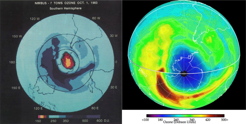
The original Ozone Hole image for October 1, 1983 presented by Bhartia et al. (1985) compared to a recent image for the same date. Though the values rendered in the original image were not accurate since correct ozone profiles were not available at that time to process the data, the basic patterns in the two images are similar.
So, the key lessons to be learned from this experience is the continuing need to collect high-quality data from in situ instruments to generate a priori profiles for satellite algorithms and validation data to confirm satellite findings. An appropriate metaphor is that satellites expand the reach of in situ measurements as a surgeon using robotic instruments does for patients in remote areas. However, as the robotic instruments cannot replace the surgeon, satellite instruments often do not replace the capabilities of in situ instruments.
For further discussion of the events described in this article the readers are referred to a recent posting by Dr. Gavin Schmidt at http://www.realclimate.org/index.php/archives/2017/12/what-did-nasa-know-and-when-did-they-know-it/.
Acknowledgements
The work described in this paper was solely funded by NASA. The data described in this paper were produced by the Ozone Processing Team (OPT) at NASA Goddard Space Flight Center led by Albert Fleig. Donald Heath, the Principal Investigator of the SBUV instrument, led the SBUV/TOMS science team. Arlin Krueger was the Principal Investigator of TOMS. The authors grateful acknowledge the contributions of late Drs. Carleton Mateer and J. V. Dave in developing the SBUV/TOMS algorithms, of our colleagues Drs. Ashok Kaveeshwar and Kenneth Klenk, and members of the OPT in producing the data described in this paper.