

1 Introduction
Thirty years after the 1987 Montreal Protocol for the Protection of the Ozone Layer (http://ozone.unep.org/en/treaties-and-decisions/montreal-protocol-substances-deplete-ozone-layer), it is important to verify that this international agreement and its subsequent amendments are achieving their goals. Indeed, Fig. 1 demonstrates that the Protocol has successfully limited chlorine in the stratosphere. At the altitudes shown in Fig. 1, hydrogen chloride (HCl) is the major chlorine-containing trace gas and its mixing ratio is closely related to the amount of chlorine (and bromine) available for ozone destruction (WMO, 2007, 2011). The fast increase of stratospheric chlorine (and bromine) from the 1960s to the late 1990s was caused by anthropogenic emission of ozone-depleting substances (ODS). This increase has clearly been stopped by the world-wide ban of ODS emissions in the early 1990s, mandated by the Montreal Protocol (e.g., WMO, 2014). Around the turn of the millennium stratospheric chlorine (and bromine) loading has peaked, and since then has been declining slowly. Assuming compliance with the Montreal Protocol, it is expected to continue decreasing in the future. While some details of the HCl evolution are complex, e.g., due to transport variations that affect the release rate of chlorine from ODS, Mahieu et al. (2014), and others are not fully understood (e.g., the double peak in 1997 and 2001 in Fig. 1), it is still clear that the Montreal Protocol has successfully curbed anthropogenic chlorine in the stratosphere (WMO, 2011, 2014). The question is now whether the chlorine decline seen in Fig. 1 since about 2000 has resulted in corresponding ozone increases over the last 10 to 15 years.
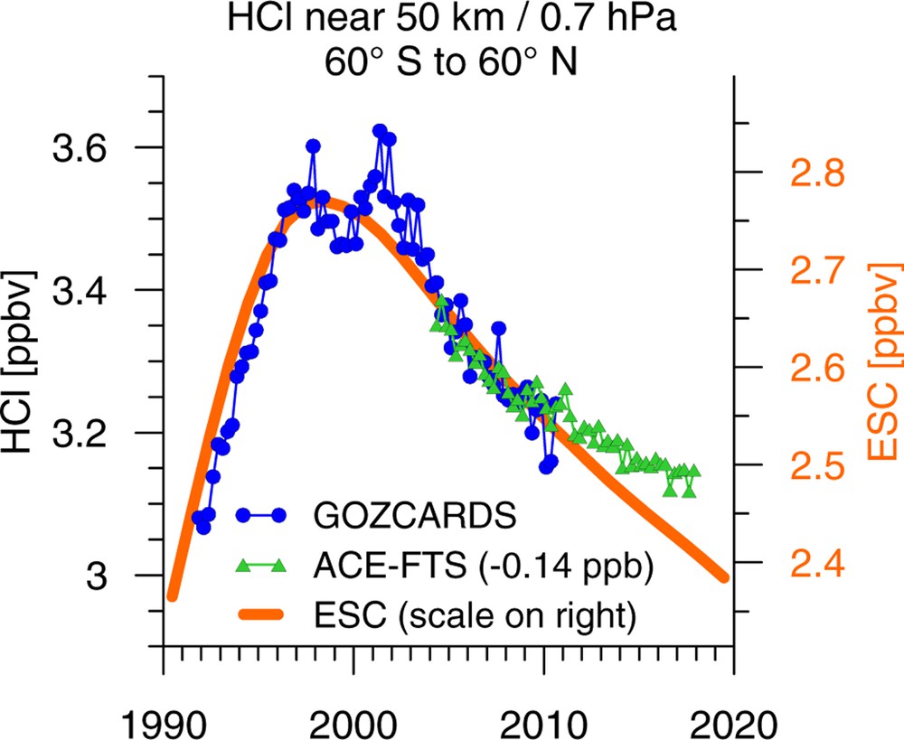
Time series of near-global (60°S to 60°N) stratospheric hydrogen chlorine (HCl) near 0.7 hPa (≈50 km altitude). The plotted Global OZone Chemistry And Related trace gas Data records for the Stratosphere (GOZCARDS) data are based on a combination of measurements from the Halogen Occultation Experiment (HALOE), Atmospheric Chemistry Experiment Fourier Transform Spectrometer (ACE-FTS) and Microwave Limb Sounder (MLS-Aura) satellite instruments (Froidevaux et al., 2015). ACE-FTS data are used to extend the time series, and are shifted to match the GOZCARDS data from 2002 to 2010. The thick orange line and the scale on the right give estimated effective stratospheric chlorine (ESC) for an age-of-air distribution with 5 years mean age and 2.5 years width (Newman et al., 2007). Updated from WMO (2011).
The search for a beginning recovery of the ozone layer requires, therefore, (a) detection of significant ozone increases in the atmosphere since the time chlorine (and bromine) peaked, and (b) attribution of a substantial part of these increases to the decline of chlorine (and bromine). In this paper, we first discuss observed ozone time-series, covering various altitude and latitude regions. We demonstrate consistency between ozone decline and increasing chlorine before the late 1990s, and ozone increases and chlorine decrease since the late 1990s, particularly in the upper stratosphere. Good agreement between observed ozone increases there with expectations from model simulations allows their attribution to declining chlorine. This provides one sign for a beginning recovery.
We then look for beginning recovery in total ozone columns. Both observational limitations and general difficulties in the detection and attribution of ozone trends are discussed. So far they have precluded the detection of a beginning recovery of total ozone columns over most of the globe. A notable exception is the region of the spring-time Antarctic ozone hole. We demonstrate that September Antarctic ozone does indeed show clear signs of a beginning recovery–as does ozone in the upper stratosphere. We conclude by summarizing these findings, and by giving an outlook on the major factors expected to control stratospheric ozone in the rest of this century.
2 Ozone time series
Fig. 2 shows a typical example of the evolution of ozone over the 1979 to 2016 period. Results are for the upper stratosphere and for northern mid-latitudes (35°N to 60°N). To a large degree, ozone is tracking the inverse chlorine evolution, e.g., as given by effective stratospheric chlorine (ESC): before the late 1990s, chlorine was increasing, and ozone was declining. Since around 2000, chlorine has been decreasing. Therefore, increasing ozone should be seen over the last 10 to 15 years. Fig. 2 indicates that, indeed, in the upper stratosphere, ozone has been increasing and is following the chlorine decline.
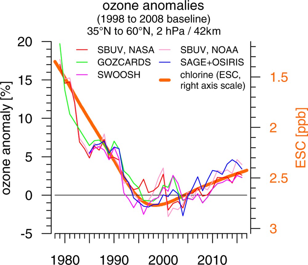
Annual mean ozone anomalies for northern mid-latitudes (35°N to 60°N) and for the upper stratosphere (42 km altitude/2 hPa pressure), from five merged satellite records: Solar Backscatter Ultra-Violet (SBUV) compiled by NASA, v8.6 MOD (Frith et al., 2017); Solar Backscatter Ultra-Violet (SBUV) compiled by NOAA, v8.6 COH (Wild et al., 2016); Global OZone Chemistry And Related trace gas Data records for the Stratosphere (GOZCARDS v2.20, Froidevaux et al., 2015); Stratospheric Water and OzOne Satellite Homogenized data set (SWOOSH v2.6, Davis et al., 2016); Stratospheric Aerosol and Gas Experiment and Optical Spectrograph and Infrared Imager System (SAGE + OSIRIS v7.0 + v5.10, Bourassa et al., 2018). Ozone anomalies for each data set are calculated with respect to its average annual cycle for the period 1998 to 2008. Thick orange curve and scale on the right: Effective stratospheric chlorine (ESC), estimated assuming an age-of-air spectrum with mean age 5 years and width 2.5 years (same as in Fig. 1, see also Newman et al., 2007). Note the inverted scale for chlorine/ESC on the right. Updated from Steinbrecht et al. (2017).
A standard approach to analyze time-series like the ones in Fig. 2 for statistically significant declining or increasing trends is multiple linear regression. The regression includes terms accounting for “anthropogenic” ozone trends, and additional terms accounting for natural ozone variability, e.g., associated with the Quasi-Biennial Oscillation, the 11-year solar cycle, stratospheric aerosol loading, transport changes and other influences (e.g., Bojkov et al., 1990; Harris et al., 2015; Newchurch et al., 2003; Reinsel et al., 2002; WMO, 2007, 2011, 2014; Zerefos et al., 2018). More complex approaches, e.g., locally weighted statistical smoothing (Krzyścin et al., 2015), dynamical linear models (Ball et al., 2018; Laine et al., 2014), or combined model-measurement approaches using simulations from chemistry-climate models (Shepherd et al., 2014; Solomon et al., 2016) are used as well. All these studies look for significant ozone increases in the last 10 to 15 years as a pre-requisite for beginning ozone recovery.
3 Ozone profile trends
Fig. 3 shows the latitude-altitude distribution of ozone trends over the 2000 to 2016 period. These trends are derived by multiple linear regression from the Global OZone Chemistry And Related trace gas Data records for the Stratosphere multi-satellite data set (GOZCARDS, Froidevaux et al., 2015). See Steinbrecht et al. (2017) for details on the trend calculations. Fig. 3 indicates significant ozone increases only in the upper stratosphere, between 35 and 48 km altitude (5 and 1 hPa pressure), from about 70°S to 85°N. At most other altitudes and latitudes, the gray shading indicates no significant ozone trends. Significance here requires that the trend is at least twice as large as its uncertainty, both resulting from the multiple linear regression. Similar ozone trends are found for other data sets, and in a number of studies (Ball et al., 2018; Bourassa et al., 2018; Frith et al., 2017; Harris et al., 2015; Sofieva et al., 2017; WMO, 2014).
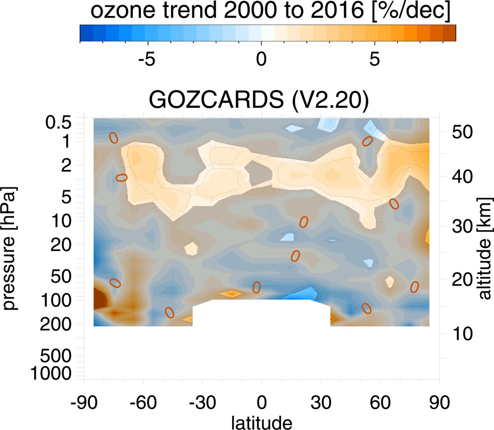
Latitude altitude/pressure cross section of observed ozone trends in % per decade from 2000 to 2016. Trends are derived from a multiple linear regression using the Global OZone Chemistry And Related trace gas Data records for the Stratosphere (GOZCARDS, v2.20) multi-satellite data set. The color scale gives the trend values. The red isoline is the zero trend line. Black isolines and gray shading show the ratio of trend to trend uncertainty. In the gray shaded region the trend is smaller than two times its uncertainty, i.e. is not significant at the 95% confidence level. The black isoline, within the unshaded region, delineates the region where trends are three times their uncertainty (99% significance). Adapted from Steinbrecht et al. (2017).
An important requirement for ozone recovery is that the observed latitude altitude pattern should be consistent with expectations from model simulations (e.g., Chipperfield et al., 2017). These incorporate our best understanding of the effects of long-term changes of ozone-depleting substances, but also of changes in greenhouse gases, especially CO2, N2O, CH4 (Eyring et al., 2010; Morgenstern et al., 2017). Fig. 4 shows ozone trends derived from model simulations in the Chemistry Climate Model Validation 2 exercise (Eyring et al., 2010; WMO, 2014). These model trends were derived similarly to the observational trends in Fig. 3. Indeed, Fig. 4 shows latitude altitude patterns of trend values, and regions of statistical significance, that are similar to the observed trends in Fig. 3. The general agreement between observed trends in Fig. 3 and simulated trends in Fig. 4 is reassuring.

Same as Fig. 3, but for simulated 2000 to 2016 ozone trends from Chemistry Climate Model Validation-2 (CCMVal2) chemistry climate model simulations (Eyring et al., 2010; WMO, 2014). Adapted from Steinbrecht et al. (2017).
Further analysis of the model simulations (not shown here) indicates that the significant ozone increases in the upper stratosphere over the last 10 to 15 years can be attributed to two major factors:
- 1) decline of anthropogenic chlorine in the stratosphere (compare Figs. 1 and 2). This reduces ozone destruction by chlorine, results in increasing ozone, and is the desired positive effect of the Montreal Protocol and its amendments (e.g., WMO, 2014);
- 2) continuing cooling of the upper stratosphere, which increases ozone by slowing gas-phase ozone destruction cycles (e.g., O + O3 → 2O2, Haigh and Pyle, 1982). This cooling is caused by increasing CO2 concentrations in the atmosphere, which increase infrared emissions from the stratosphere to space and reduce infrared heating from the troposphere.
Both effects contribute roughly equally to the increase of upper stratospheric ozone seen in Figs. 2 to 4 over the last 10 to 15 years (e.g., Shepherd and Jonsson, 2008; WMO, 2014). These observed ozone increases in the upper stratosphere are, therefore, a strong sign for ozone recovery and for the success of the Montreal Protocol. Ironically, increasing CO2 concentrations, which cause climate change, contribute to this recovery and enhance it.
The simulations in Fig. 4 suggest ozone increases almost everywhere, except for the extended tropical lower stratosphere, from 30°S to 30°N and between 100 and 20 hPa (17 and 26 km). Ozone decreases in this region in the simulations (blue colors in Fig. 4) are also present in observational data sets (Randel and Thompson, 2011; Sioris et al., 2014; to a lesser degree also in Fig. 3). The simulations attribute this tropical decline to increases in the strength of the Brewer-Dobson circulation (Aschmann et al., 2014; Butchart et al., 2006, 2010; McLandress and Shepherd, 2009), which are ultimately caused by increasing CO2 and other greenhouse gases. This results in enhanced upwelling of ozone poor air in the tropical lower stratosphere, and also in enhanced poleward and downward transport of ozone rich air in the extra-tropics. The latter should enhance positive ozone trends in the extra-tropics. In the tropics, however, the simulated changes in the Brewer-Dobson circulation reduce total ozone columns, because ozone decrease in the lower stratosphere is larger than ozone increase in the upper stratosphere (e.g., Hegglin and Shepherd, 2009).
4 Limitations for trend detection
A number of factors are necessary before significant trends can be detected:
- 1) the magnitude of the trend (signal) must be large compared to atmospheric and observational “noise”. Fig. 4, for example, indicates that large and significant (relative) ozone increases are expected in the upper stratosphere (near 43 km/2 hPa) and at higher latitudes, a region with moderate atmospheric variability. Even larger ozone increases are expected for the ozone hole region in the lower stratosphere above Antarctica (90°S, 10 to 20 km/200 to 50 hPa). However, large natural ozone variations in this region mask the trend and make it non-significant, at least in the annual mean (gray shading in Figs. 3 and 4). The same is generally the case over much of the lower stratosphere (below 20 hPa or 25 km), where trends are usually not significant (large gray shaded regions in Figs. 3 and 4);
- 2) the considered period (sample) should be as long as possible. Trend uncertainty typically scales with n−1.5 (e.g., Weatherhead et al., 2000), where n is the number of (independent) data points, e.g., months or years. Record length and statistical independence/low auto-correlation of the data points, therefore, play important roles. Long records are also necessary to account correctly for other ozone variations, e.g., those due to the 11-year solar cycle;
- 3) accuracy and long-term stability of the observing system should be high, typically of the order of 1% per decade, or better. In Fig. 2, for example, time series and trends from the different satellite records differ only by 1 to 2% per decade, but drifts exceeding 3% per decade have been reported for some data sets (Hubert et al., 2016). In Fig. 2, the possible drifts are smaller than the 4% ozone increase since 2000 itself. However, with comparable instrumental uncertainty and stability, a smaller ozone increase might not be significant;
- 4) uncertainties due to data sampling (Damadeo et al., 2018; Millán et al., 2016), data merging (Frith et al., 2017), trend estimation (Reinsel et al., 2002), etc. must all be small, again typically less than 1% per decade.
Weatherhead et al. (2000) discuss the implication of limitations 1 and 2 for the detection of recovery trends in total column ozone. Their results indicate that in most regions it will take at least 20 to 30 years before statistically significant total column increases can be detected with good confidence (2σ/95%, or higher). A key issue in this respect is the slow decline of stratospheric chlorine since the late 1990s, which is much slower than the fast chlorine increase before the mid-1990s (see ESC curves in Figs. 1 and 2). The ratio of the respective slopes is roughly 3:1 or 4:1. Everything else being equal, it will take several times longer to detect ozone recovery, compared to the 10 or 15 years it took to detect ozone decline before the mid-1990s.
Limitations 3 and 4 pose additional difficulties for detecting ozone recovery. Hubert et al. (2016), for example, show that it is difficult to determine the long-term stability of limb scanning satellite instruments and of ground-based ozone profiles with accuracy better than 3% per decade. In particular, multiple independent instruments are absolutely necessary to have any information about accuracy and long-term stability. If there were only one or two lines (instruments) in Fig. 2, it would be impossible to make statements about their stability and accuracy. Most of the limitations under 3 and 4 are currently being investigated by the Long-term Ozone Trends and Uncertainties in the Stratosphere (LOTUS) initiative, see http://www.sparc-climate.org/activities/ozone-trends/.
5 Total ozone column trends
A major driver for the Montreal Protocol was the fear that global ozone decline would result in large increases of harmful ultra-violet (UV) radiation at the Earth's surface (e.g., Hegglin and Shepherd, 2009; WMO, 2007). UV radiation at the surface is controlled by changes in the total ozone column, no matter where they occur in the ozone profile. In Fig. 5 we, therefore, present the evolution of near-global total ozone columns. The observations clearly show significant decline by about −1.8% per decade from 1980 until the mid-1990s. This decline was caused by increasing chlorine (and bromine) from ODS emissions. The Montreal Protocol, together with its amendments, has successfully stopped these emissions and ozone has responded. Since the late 1990s, near-global ozone columns have not declined further, and have remained more or less stable.

Annual mean total ozone columns for the 60°S to 60°N latitude band (near-global), from five data sets. The World Ozone and UV Data Center data set (WOUDC) are compiled from ground-based observations by Dobson- and Brewer spectrometers and filter instruments. Solar Backscatter Ultraviolet (SBUV Version 8.6) NASA and NOAA are both merged data sets, based on the series of SBUV/2 satellite instruments since 1978. The GSG and GTO merged data sets are based on the Global Ozone Monitoring Experiment (GOME), Scanning Imaging Absorption Spectrometer for Atmospheric CHartographY (SCIAMACHY) and GOME/2 satellite instruments since 1996. GTO additionally uses the Ozone Monitoring Instrument (OMI) satellite instrument. True global mean data are not available, because the observations are limited to the sunlit part of the globe, and are not available polewards of 60° in winter. The thick orange line and the black trend lines show results of a multiple linear regression fit (MLR) to the SBUV V8.6 NASA data set (MLR NASA). Independent linear trends were used to describe ozone trends before and after the turnaround of stratospheric chlorine and bromine in the mid- to late 1990s. The resulting independent linear trend lines do not necessarily connect. Numerical trend values and their 2σ uncertainties are given in the top part of the plot. The regression fit explains 92% of the observed variance (r2 = 0.92), uses 13 predictor time series (m = 13), is based on 38 annual mean data points (n = 38), and has a mean square error of 1.3 Dobson Units (χ = 1.3 DU). Adapted from Weber et al. (2018).
Near-global total ozone in Fig. 5 is a good example for the trend detection limitations discussed in the previous section. Limitation 1: the expected increases since the late 1990s are quite small, only 0.4 to 0.6 % per decade. This makes them difficult to detect, even though atmospheric noise is also small for the near-global averages in Fig. 5 (because regional transport variations tend to cancel out in the large scale average). The time series is also almost 40 years long (limitation 2) which should help with trend detection. The multiple linear regression fit in Fig. 5 (thick orange line) can indeed account very well for long-term changes and inter-annual variations, including the 11-year solar cycle (explained variance R2 = 92%). While the decline from 1980 to the mid-1990s is statistically significant (linear trend −1.8 ± 0.7% per decade, 2σ uncertainty), the possible increase since the late 1990s is too small and remains statistically insignificant at this point (+0.2 ± 0.3% per decade, 2σ). This is consistent with expectations from Weatherhead et al. (2000), who show that near global total ozone might show early signs of increasing trends, but not before 2015 to 2020.
In addition, differences between the data sets in Fig. 5 are large enough (limitations 3 and 4) to be comparable to the expected trend since the late 1990s, even though these differences are small in absolute numbers, only 2 to 4 Dobson Units (DU) or ∼1%, between the ground-based data from the World Ozone and UV Data Center (WOUDC, red line) and the satellite-based Solar Backscatter Ultra-Violet data sets (SBUV, blue lines) in 2016. All this makes detecting a significant increase for near-global total ozone since the late 1990s challenging. Still, the small and insignificant increase since the late 1990s in Fig. 5 is not inconsistent with expectations.
Generally, total ozone columns are less sensitive to changing chlorine than ozone in the upper stratosphere. At individual latitudes, total ozone columns are also affected more by transport variations than the near global mean in Fig. 5, particularly by transport variations of ozone in the lower stratosphere. This atmospheric “noise” generally increases with latitude and often masks small chlorine related trends in latitude resolved total ozone columns (see also the large gray regions with non-significant trends in Figs. 3 and 4). Chemistry-climate or chemistry-transport models can help to better disentangle chemical ozone change from transport related ozone change (Chipperfield et al., 2017; Shepherd et al., 2014; Solomon et al., 2016). Chipperfield et al. (2017), for example, find a model simulated “chemical” recovery of +12 DU by 2016 for southern hemisphere mid-latitudes (60°S to 35°S) since the late 1990s. However, this chemical increase appears to be masked by transport related ozone changes of −10 DU over the same time period. Both effects together result in a small overall increase of only +2 DU, consistent with the lack of clear recovery signs in southern mid-latitude observations reported, e.g., by Weber et al. (2018). Overall, total ozone columns at most latitudes show behavior similar to the near global means in Fig. 5, and do not yet show statistically significant total ozone increases since the late 1990s (e.g., Weber et al., 2018).
Long-term changes in tropospheric ozone columns may also play a role. Shepherd et al. (2014), for example, suggest that a long-term decline in tropical stratospheric ozone, due to chlorine increases and enhanced ascent in the Brewer-Dobson circulation, has been compensated by increases in tropospheric ozone, so that tropical total columns have remained constant–in contradiction to many other model predictions which simulate long-term declines of tropical stratospheric and total column ozone (Eyring et al., 2010; WMO, 2014). A recent paper by Ball et al. (2018) argues that ozone in the lowermost stratosphere (below 20 km/70 hPa, and from 60°S to 60°N) has been continuing to decline since the 1980s. This might also be indicated by the (albeit non-significant) lower stratospheric trends in Fig. 3. According to Ball et al. (2018) lower stratospheric decline has been compensated by increases in tropospheric ozone. Lower stratospheric decrease and tropospheric increase might then combine to the more or less constant total ozone columns since the late 1990s (e.g., in Fig. 5), and might explain the current lack of clear increases in total column ozone. Reliable observations showing such tropospheric increases, however, are missing, and the recent Tropospheric Ozone Assessment Report (TOAR) found large disagreements in the magnitude and even in the sign of tropospheric column ozone trends (Young et al., 2018). Certainly, these questions need to be investigated further in the near future.
6 Recovery over Antarctica?
The Antarctic ozone hole is the clearest and most prominent manifestation of ozone destruction by anthropogenic chlorine and bromine (WMO; 2007, 2011, 2014). Antarctic total ozone columns are more sensitive to chlorine (and bromine) than tropical or mid-latitude ozone columns (e.g., those in Fig. 5). Antarctic spring, therefore, is a good region to search for ozone increases and for beginning recovery. Fig. 6 shows the evolution of total ozone columns above Antarctica in September, the month when much of the chemical ozone depletion in the ozone hole occurs. Again, multiple linear regression can account for a large fraction of the observed variations and trends (R2 = 0.82). The regression shows significant ozone decline from 1980 until the late 1990s (−12.2 ± 10.7 % per decade, 2σ uncertainty). This is seven times larger decline than for near-global total ozone in Fig. 5. The regression also shows significant ozone increase since the late 1990s (+10.1 ± 6.9% per decade, 2σ).
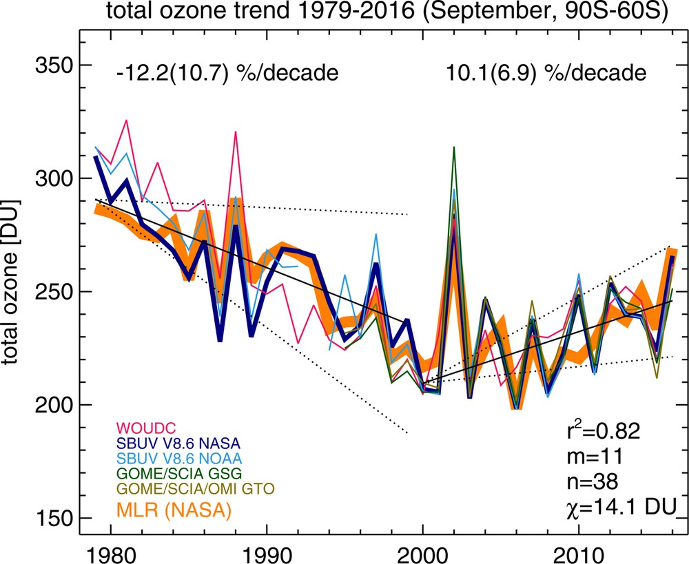
Same as Fig. 5, but for spring-time total ozone columns above Antarctica in September (90°S to 60°S). Adapted from Weber et al. (2018).
As mentioned before, the decline of chlorine (and bromine) since the late 1990s is three to four times slower than their previous increase. Consequently, the slope of increasing total ozone since the late 1990s in Fig. 6 should also be three to four times smaller than the previous declining slope: the–12.2% per decade decline of September total ozone columns before the late 1990s in Fig. 6 should have turned into a 3 to 4% per decade increase since the late 1990s. The observed increase, +10.1% per decade in Fig. 6, however, is two to three times larger than this. Apart from declining chlorine (and bromine), therefore, transport variations must have played a major role as well.
Consistent with this, a recent chemistry-climate model based study indicates that chlorine decline explains about half of the ozone increase observed in Fig. 6, while inferred transport changes are necessary to explain roughly the other half (Solomon et al., 2016). In some years, increased stratospheric aerosol from volcanic eruptions is important as well. The eruption of Mt. Calbuco in Chile, for example, is thought to have increased the size of the 2015 ozone hole by 25%. Apart from Solomon et al. (2016) and Fig. 6, a number of recent studies provide evidence for increasing ozone above Antarctica in spring, connected to the decrease of chlorine. The vertical profile trend study by Kuttippurath and Nair (2017), for example, reports substantial ozone increases between 10 and 20 km altitude, based on ozone-sonde data, and attributes at least part of the increases to declining chlorine. De Laat et al. (2017) use ozone mass deficit derived from satellite observations and find significant ozone increases for Antarctic springtime based on this measure. Evidence is mounting for a beginning recovery of the Antarctic ozone hole!
7 Conclusions
A number of signs for a beginning recovery of the ozone layer have been observed in recent years. The clearest signs, so far, are ozone increases over the last 10 to 15 years in the upper stratosphere, and a decrease in the severity of the Antarctic ozone hole in September. These are the stratospheric regions most sensitive to anthropogenic chlorine. At the same time, it is certain that the significant ozone decline from the 1960s to the 1990s has leveled off. The world-wide ban of ozone-depleting substances (ODS) by the Montreal Protocol and its amendments has been successful!
Expectations are that ODS concentrations will keep decreasing, and that the ozone layer will continue to recover. However this process will be slow, much slower than the fast ozone decline from the 1960s to the 1990s. Ozone concentrations as in the 1960s are not expected before 2040 or 2050 (WMO, 2014). By that time, ODS concentrations should have declined substantially, and expected increases in other trace gases will become important for the ozone layer (WMO, 2014). Increasing N2O and CH4 will affect ozone production and loss cycles, with N2O generally decreasing ozone and CH4 generally increasing ozone. Model simulations indicate that ozone changes due to these gases will likely become comparable in magnitude to the past ozone decline due to ODS (e.g., Li et al., 2008; WMO, 2014). Increasing CO2, stratospheric cooling, and climate change have also affected and will continue affecting the ozone layer and global ozone transport in the Brewer–Dobson Circulation (Butchart et al., 2010; WMO, 2014). Hossaini et al., 2017 show that substantial future increases in short-lived chlorine-containing gases like dichloromethane could also slow ozone recovery. With all these competing and potentially substantial effects, it seems imperative that accurate ozone and other trace gas measurements are continued throughout the coming decades. Models also need to be developed further. The combination of observations and model simulations remains essential for understanding the past and for predicting the future. Both are necessary to ascertain that the recovery of the ozone layer continues over the next decades, and that the 30-year-old Montreal Protocol and its amendments remain effective.
Acknowledgements
The authors are very grateful to Lucien Froidevaux (JPL-Caltech), Ray Wang (Georgiatech), and John Anderson (Hampton University) for contributing the GOZCARDS data sets used here. The authors also thank Peter Bernath and Anton Fernando (Old Dominion University) for providing the updated ACE–FTS hydrogen chloride record.