


 CC-BY 4.0
1. Introduction
Magnetic and gravity data inversion is used to estimate the susceptibility and density distribution in the underground. Several inversion techniques exist for potential fields [Boulanger and Chouteau 2001, Camacho et al. 2000, Li 2001, Li and Oldenburg 1996, 1995, Moraes and Hansen 2001]. The magnetic and gravity data inversion can be considered to be linear or nonlinear. In some cases, the question is only of looking for the block susceptibilities and densities, because the geometries are fixed. In other cases, the question is of determining the geometries [Camacho et al. 2000, Montesinos et al. 2003], all this these inversion methods can lead to linear and non-linear approaches depending on the choice of the method or on the problem to be solved. The other difficulty encountered in inversion is the non-uniqueness of the solution, this is a problem inherent to all inversions.
The minimisation algorithm used in the majority of cases comes from the algorithm developed by Beiner [1970]. The principle is to construct an error function. At each iteration of the inversion, the geologic model is calculated. The error function evaluates the difference between the measured data and the model response. As long as this difference remains large, the model parameters are varied one after the other until a set of parameters minimizing the error function is found. In this way, this approach is repeated for a number of iterations until one obtains the model whose response best satisfies the data. This principle can be compared to the analysis of a topographic surface [Beiner 1970, Fischer and Le Quang 1981] looking for the lowest point. Each iteration helps to descend along this topography and to converge towards the goal that represents the final model. A smoothing term is added to the previous approach to prevent the model from having unrealistic contrasts, however, the approach used in our work was based on a linear inversion. The linear inversion techniques are formed by the so-called gradient-based methods. The problem to be solved can be significantly reduced by the linearization of the forward problem. By linearization, the response functions can be greatly simplified. Linear inversion methods are based on the solution of sets of linear equations, which can be solved relatively fast. These prevailing methods are used for several geophysical problems, the main point of these methods is the linearization of the forward problem.
The minimum-structure, voxel-based inversion consist to invert the gravity data directly to recover a minimum structure model, the earth is modelled by using a large number of rectangular cells of constant density, and the final density distribution is obtained by minimizing a model objective function subject to fitting the observed data. The model objective function has the flexibility to incorporate prior information and thus the constructed model not only fits the data but also agrees with additional geophysical and geological constraints. A depth weighting is applied in the objective function to counteract the natural decay of the kernels so that the inversion yields depth information. Applications of the algorithms to synthetic and field data produce density models representative of true structures [Li and Oldenburg 1998]. The parameters depth weighting depends on the discretization of the model but they are calculated easily. When the gravity data are known to be produced by positive density contrasts, this can be incorporated into the inversion and it has been shown to improve the solution. Applications of this method to synthetic data sets have produced density models representative of the true structures, and the inversion of field data has produced a density model consistent with the geology [Li and Oldenburg 1998].
In order to process the data and do an unconstrained inversion, many processing steps were conducted using Geosoft Oasis montaj and Voxi Earth Modelling™. They are based on Cartesian cut cell for cloud data inversion. The starting point is unconstrained inversion with data processing and analysis, up to the full inversion.
2. Geological context
2.1. Geological framework
The Jebilets-Guemassa metallogenic province consists of two large mining complexes. These districts are located in the western Moroccan meseta, respectively south-west and north of Marrakech (Figure 1A). The central Jebilets zone is characterised by a Hercynian cycle continuum [Bordonaro 1983, Huvelin 1977]. During this cycle, this zone experienced intense hydrothermal alteration [Ben Aissi 2008, Essaifi 1995] and strong magmatic activity [Aarab 1984, 1995, Bordonaro 1983, Huvelin 1977, Jadid 1989]. Thus, the acidic and basic intrusions that form the sub-contemporary bimodal plutonism [Essaifi 1995], are composed of several meters thick bodies, organised in NNE “submeridian” lineaments, parallel to the Hercynian structures [Ben Aissi 2008, Essaifi 1995]. These intrusions contain visible metallotects at the surface, within the iron caps, distributed in three major axes. Around the magmatic bodies, regional deformation and contact metamorphism are developed [Bordonaro 1983, Huvelin 1977, Zaim 1990], which has profoundly altered the primary structures and the associated deposits. The Guemassa massif is composed of a tectonic block included in the plioquaternary overburden. It is composed of sedimentary and volcano-sedimentary terrains, which belong to the Upper Visean-Namurian age [Hathouti 1990, Hibti 1993]. The Hercynian basement is covered with Plio-quaternary tabular sediments, attached to the north-atlasic half-horst group [Zouhry 1999]. The volcanic acid series are well developed with iron caps [Hathouti 1990]. They contain distal and proximal tuffs as well as lava flows [Hibti 2001, Hibti 1993].
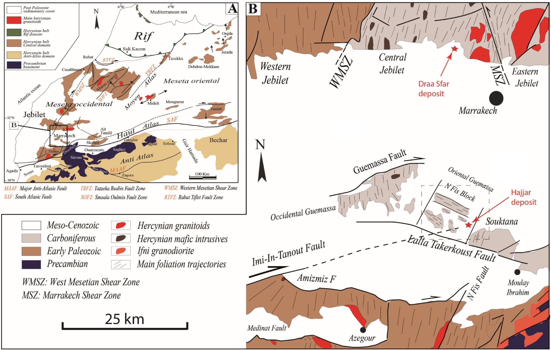
A: Structural map of Morocco showing the major bounding-fault domains. The arrows indicate the sense of shears for the late Variscan structures according to [Admou et al. 2018]. B: Geological and structural map of the central domain of the Hercynian belt according to [Admou et al. 2018].
2.2. Mineralization
This part is taken from [Jarni et al. 2015], who describe in details the Hajjar mineralisation. The geological data analysis shows that it is a polymetallic volcanogenic massive sulfide ore deposit, with ore resources of 18 million tonnes with 4–10% zinc, 2–4% lead, 0.4–0.8% copper and 60 ppm silver. The sulphide cluster has a dominant pyrrhotite grained texture (90 to 95%) mineralised with sphalerite, chalcopyrite, native copper and silver galena. This orebody is elongated NNW-SSE, with a 250 to 500 m longitudinal extension, a 50 to 250 m lateral extension and a thickness of 40 to 70 m (Figures 2, 3). The mineralisation is hosted in Carboniferous volcanic, volcano-sedimentary formations. It is located immediately on the rhyolitic dome roof, with clear alteration zones. The orebody is covered by an iron cap, which has a very rich cementation zone of native copper (40%) and of lead with a silver galena vein of 10 to 20 cm [Jarni et al. 2015].
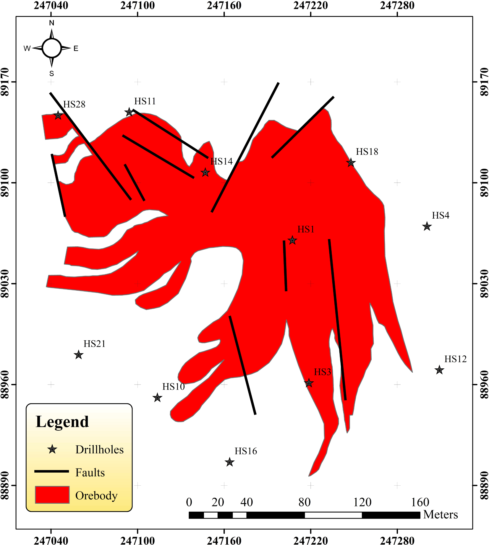
Drillholes disposition from the surface and orebody geometry at level −235 m modified from [Hathouti 1990].
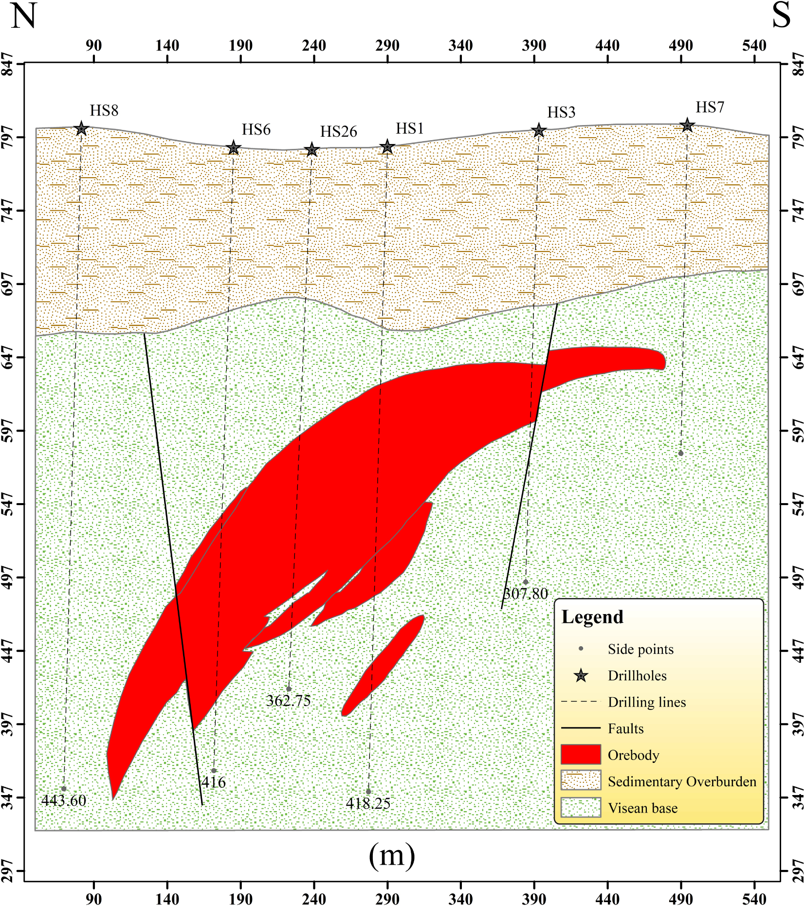
Section of Hajjar sulphide mineralization from the drilling data (Tables 1 and 2).
3. Materials, methods and calculation
3.1. Geophysical investigation and data collection
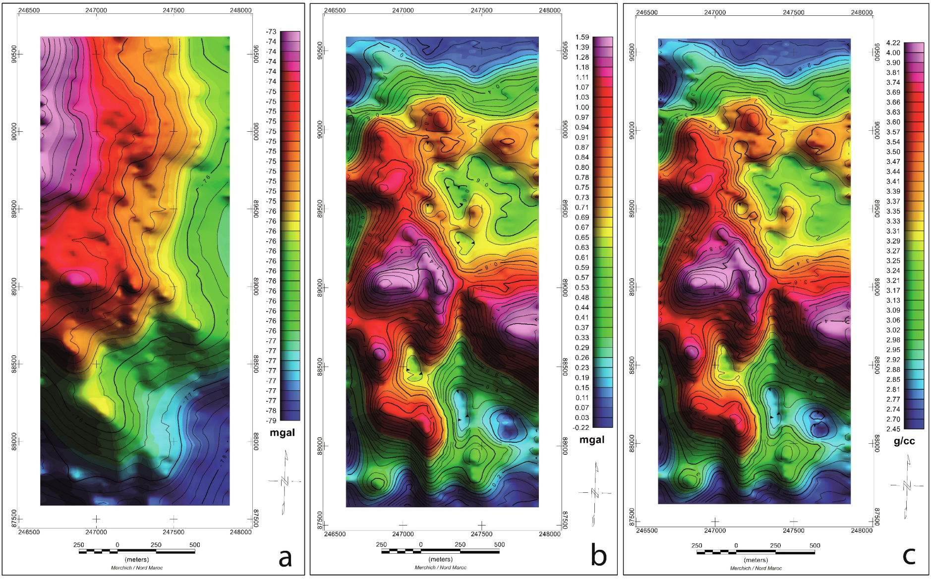
Completing the geophysical gravity investigation presented by Soulaimani et al. [2017], we added geophysical magnetic measurements. Hence the importance of using gravity and magnetic data together to locate hidden sulphide clusters at depth. After the discovery by the HS1 drilling of the Hajjar sulphide mineralization (Figures 2, 3), a detailed gravity and magnetic survey was carried out by the Geophysical Survey of the Moroccan Directorate of Geology in May 1984. The area extension is 3.2 km long and 1.6 km wide. In total, 1089 gravity stations and 1210 magnetic stations were used (Figure 4a). The station spacing is 25 m. However, the spacing between the profiles is 200 m except for the 5 central profiles, for which the spacing is reduced to 100 m (Figure 4a). The data acquisition was carried out using a Lacoste and Romberg gravimeter and a caesium magnetometer, with a resolution of 0.01 mGal and 1 nT, respectively.
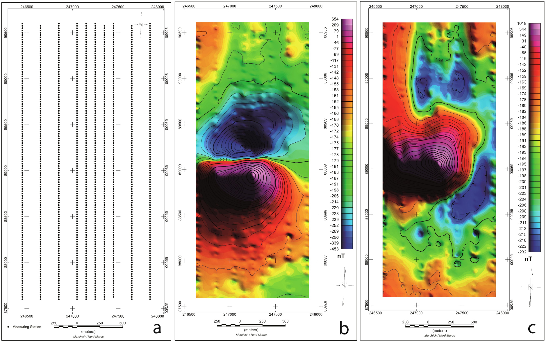
a: Profiles of gravity and magnetic survey lines, b: residual magnetic anomaly map, c: reduced-to-the-pole residual magnetic anomaly map.
3.2. Methodology
3.2.1. Magnetic data
To study the magnetic anomaly, the IGRF field was removed, the residual magnetic field is computed as the difference between the total field and the calculated IGRF. Finally, the residual magnetic data was reduced to the pole using an inclination of 46° N and a declination of −7.40° W. The transformation is done in the frequency domain by using the filter operator [Grant 1972], the interpolation has been performed by the minimum curvature gridding method.
3.2.2. Gravity data
The Hajjar gravity data that we were able to process included all the detailed calculations made by the Geological Survey of the Geology Directorate of Rabat. In addition, we created a database that contains the Bouguer anomaly for a regional density of 2.67 g∕cm3. The 2.67 g∕cm3 and 2.3 g∕cm3 are the densities commonly used for gravity surveys in Morocco.
The 2.67 g∕cm3 density was used for the Hajjar area because it had not been used in previous studies, and the Bouguer correction depends on the dominant bedrock geology/composition for the area (a volcano-sedimentary formation), in addition, the maximum changes in elevation in the area covered by the gravity data is 117 m, which is small compared to the thickness of the sedimentary cover (124.4 m) and the orebody depth (158 m) [Bellott et al. 1991]. The average density of the sedimentary cover (about 2.67 g∕cm3) was used.
Therefore, one of the first calculation steps is to individualise the interesting anomaly, so as to propose density models that can account for it. For this purpose, we first defined the regional field. Several techniques can reveal the appearance of a regional anomaly. In order to do so, we decomposed the signal by linear separation, or by a functional Fourier transform that represents the Bouguer anomaly. As part of our study, we are interested to locate anomalies of a few tenths of mGal. The technique that we used for data processing was initially selected after testing several methods. It consists of a linear separation. However, the residual field (RES) is obtained from the subtraction of the obtained regional field (REG) from the Bouguer anomaly (BA) similar to the method used by El Azzab et al. [2019], the interpolation has been performed by the minimum curvature gridding method.
3.2.3. Excess mass (Gauss’s law)/apparent density filter
Gauss’s law states that the total mass in a region is proportional to the normal component of the gravitational attraction integrated over the closed boundary of the region [Jackson 1996]. Among the most common geophysical applications of this concept is the approximation of excess mass beneath a surface over which the normal component of gravity is known [Hammer 1945, Jackson 1996]. Given a volumetrically constrained mass, no other assumptions regarding its depth, shape or density distribution are necessary. This is with the exception, however, that the studied mass must be small compared to the overall dimensions of the study area [Jackson 1996]. Some complications do arise with the application of Gauss’s law in this manner. Gravity data over an infinite plane does not exist, and therefore, the best proxy is to utilize a dataset that extends markedly beyond the limits of any major sources of interest. Complete source isolation is unfortunately not possible in the natural world. For this reason, the separation of the gravitational anomalies of interest from other local and regional sources is often complex [Jackson 1996].
Gauss’s law allows to calculate the total excess mass that produces a gravity anomaly, regardless of the distribution of this mass. Green found this solution to the excess mass within the Earth using a hemisphere for the hypothetical surface, S [Siqueira et al. 2017]. Assume that the top of the hemisphere is the surface of the Earth (z = 0). Then the surface integral can be divided into the top and the hemisphere [Connor and Connor 2009]. By assuming that the radius of the hemisphere is extremely large, some adjustments are made with the limits of integration to simplify the problem, in practice, the anomalous mass is found by numerically integrating the gridded gravity data across an area [Connor and Connor 2009]:
a: Bouguer anomaly map for the density of 2.67 g∕cm3, b: map of the residual gravity anomaly, c: density map.
Nevertheless, an apparent density filter calculates the apparent density of the ground that would give rise to the observed gravity profile. The density assumes that the gravity profile is due to a set of rectangular prisms with a top at the level of observation of the gravity profile, a bottom at depth t, and an infinite strike length; we must supply the thickness of the earth model and the background density [Gupta and Grant 1985]:
3.2.4. Inversion by VOXI earth modelling™
Voxel-based modelling and inversion has become a familiar tool over the last two decades, due to its dramatically reduced computing costs, and to the fact that the exploration industry attempts to interpret increasingly complex geophysical data associated with deeper targets. The simplicity of voxel-based representations of the earth makes them appealing. They are easily understood and easily programmed, easily displayed, and conform to current computer architectures. However, they have one significant shortcoming: they are not well suited for representing the geological features common in exploration projects, because geological features are often described by surfaces [Ellis and MacLeod 2013].
VOXI Earth Modelling™ is a Geosoft Oasis Montaj cloud and clustered computing module that allows the inversion of geophysical data (e.g., gravity, magnetics) in 3D. It uses a Cartesian Cut Cell (CCC) inversion algorithm developed by Ingram et al. [2003]. The algorithm has been simplified by Ellis and MacLeod [2013] in order to represent geological surfaces with greater accuracy. Inversions can be made as unconstrained Roy et al. [2017]. Gravity and magnetic data (ground or airborne data, total field or gradient measurements) can be inverted using different methods Barbosa and Pereira [2013], Ellis and MacLeod [2013], Farhi et al. [2016], Ingram et al. [2003].

a: Section of the magnetic inverse model, b: section of the gravity inverse model, c: magnetic inverse model relative to the mineralisation, d: gravity inverse model relative to the mineralisation.
The data source can be provided in either Database or Grid format. For our case, we used the residual grids for above cases, gravity and magnetic data as sensor grid. Therefore, we were obliged to define the sensor elevation as grid files for the elevation sensors and choose the number of samples per cell. Initially, all effects such as motion, terrain, tide, regional field, etc. must be removed prior to modelling for both cases “gravity” and “magnetic data”. Secondly, we fixed the fit criterion (model sensitivity) to fit the data until the difference between the model prediction (the fit) and the measured data is on average less than the Fit criterion. Increasing the fit criterion increases the smoothing of the inversion results. For fitting methods, we can use several options like absolute errors, relative error or fraction of standard deviation [Bhattacharyya 1965, Dampney 1969, Dransfield 2007, Pedersen and Rasmussen 1990]. We chose the default value familiar with the geophysicists that equals 5% of the data standard deviation. For our case study, the standard deviation of gravity data equals 0.008504 mGal and that of magnetic data equals 8.94 nT.
4. Synthesis and results
4.1. Magnetic maps
The Hajjar residual magnetic anomaly (Figure 4b) has a bipolar shape with a minimum to the north and a maximum to the south. Its east-west longitudinal axis is 1.4 km long. The residual magnetic anomaly amplitude is 654 nT. One can see from the magnetic residual anomaly map that this anomaly exists in a quiet magnetic context, which was a favourable factor for its identification. In order to be able to define the mineralised body and compare it with the gravity anomaly, we have computed the reduced-to-the-pole (RTP) magnetic anomaly.
The RTP map (Figure 4c) reveals a very important unipolar magnetic anomaly, that is coincident with the deposit displaying a maximum amplitude of 1018 nT. This maximum can be interpreted as located over the deposit center (hence the reason for positioning there the HS1 drilling during the exploration phase in the 80s and 90s).
4.2. Gravity maps
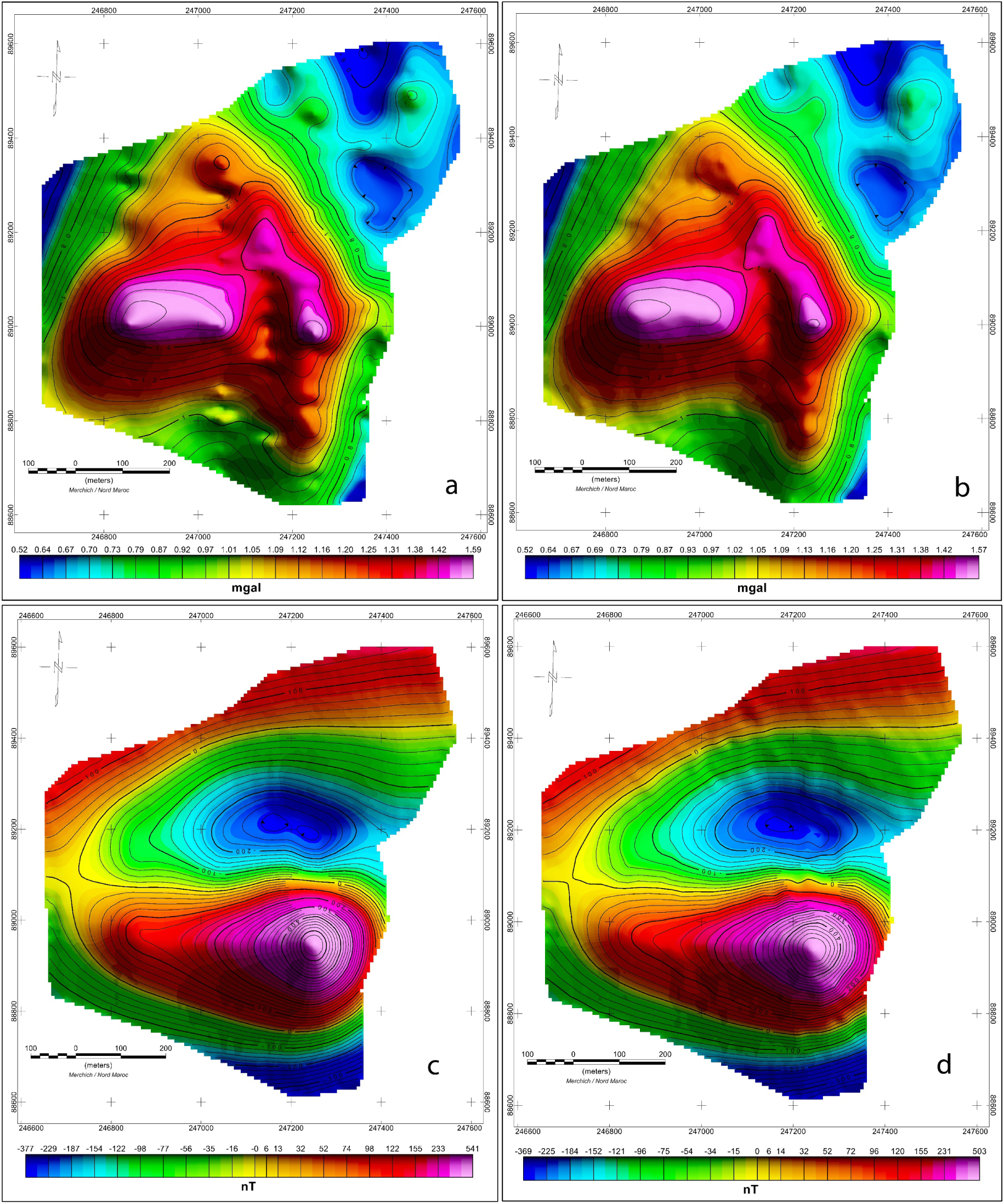
The orebody residual anomaly maps. a: Gravity, c: magnetic. Accompanied by the inverse models responses. b: Gravity response, d: magnetic response.
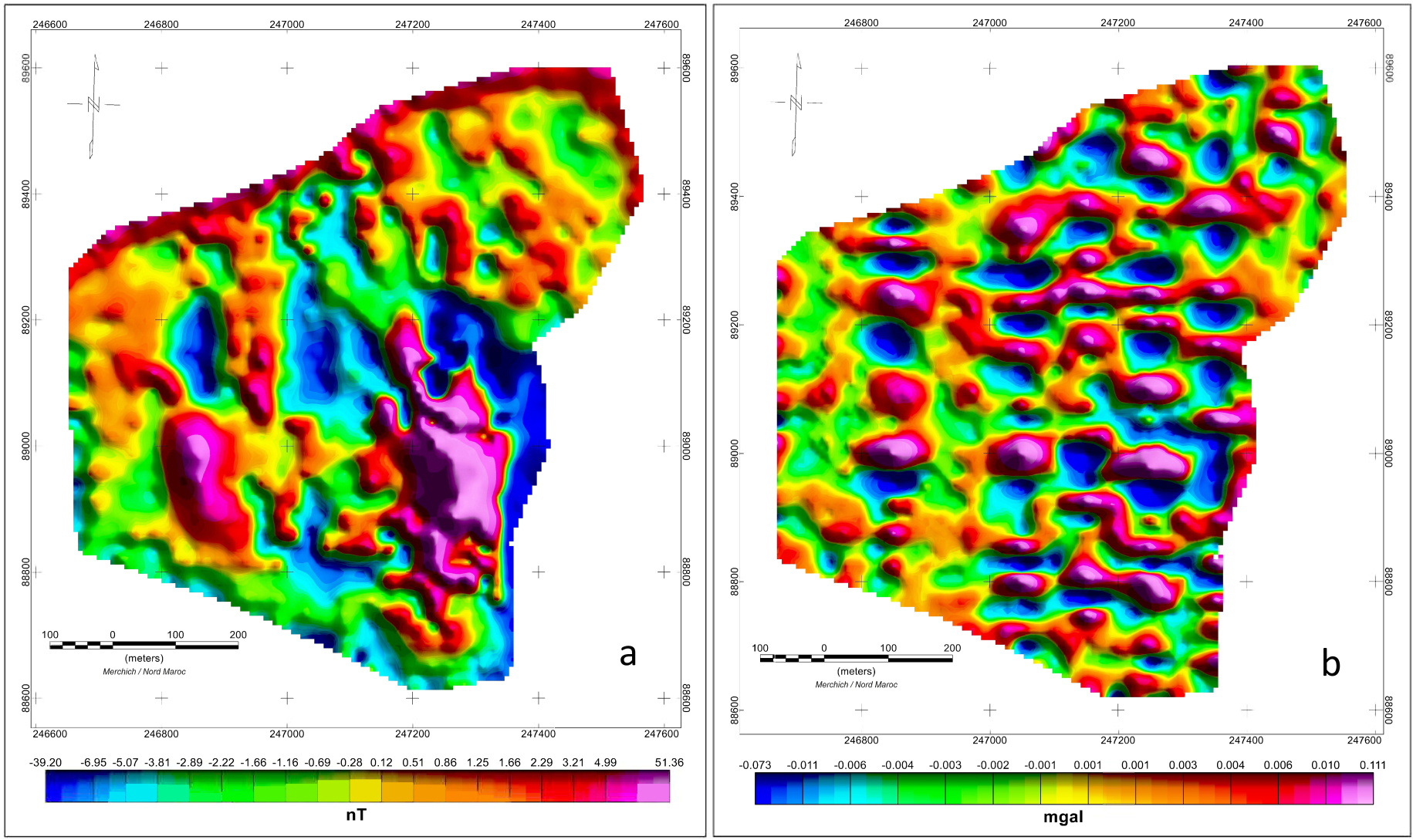
Map of the differences between the observed and computed data, for both. a. Magnetic data, b. gravity data.
We have displayed the Bouguer anomaly as a contoured colour map. This Bouguer anomaly map (Figure 5a) shows a north-south positive anomaly located to the northwest. This map is displayed with 0.2 mGal-spacing contours. The general plot shape shows negative anomalies oriented roughly SE-NW with a gravity gradient increase from the southeast to the northwest. Several anomalies are highlighted with different wavelength and amplitude related to the geological structures whose dimensions and densities are variable.
The Bouguer anomaly map does not allow drawing an interpretation of the shallow structures since a regional field effect is obvious. If this map requires interpretation, the large positive field range in the north-western part can be explained by the regional effect due to regional geological structures. In our case, it can be interpreted as a sedimentary cover thickening in the south-eastern part and thinning in the north-western part.
On the residual gravity anomaly map (Figure 5b), we found a very important positive anomaly in the left center with an amplitude of 1.59 mGal. It has a circular shape with two elongations: an E-W directional extension and a NW-SE direction bordered by mid-amplitude and less narrow anomaly bands. This anomaly occupies an area of 333,000 m2. By analysing the residual gravity anomaly map (Figure 5b), we were able to identify the positive anomalies.
4.3. Excess mass/density map
Following the residual-regional part of the data set, using linear separation, an area immediately surrounding the Hajjar gravity anomaly was selected for the purpose of performing an excess mass calculation. To effectively perform this calculation, the gravity data must first be interpolated on a regular grid, step already done.
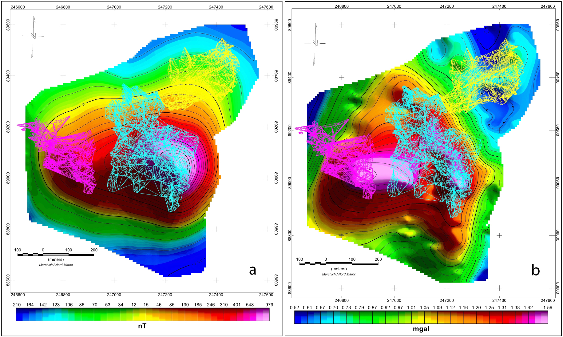
Layout of the three orebodies deposit. a: RTP magnetic anomaly. b: Residual gravity anomaly.
A threshold (“background”) gravity value is then visually determined from the gravity map. This background value, in the case of the Hajjar anomaly, was determined to be approximately 0.52 mGal. Utilizing a personal software to perform a numerical integration of the gridded gravity data across the selected area of interest, the anomalous mass is determined by subtracting the assigned background value from each grid point which coincides with the ore body, then summing up all the values together. The sum is subsequently multiplied by Δx⋅Δy∕2πG.
Based on the selected background value of 0.52 mGal, the excess mass calculated for the Hajjar anomaly is 7.32 × 10⁹ kg:
4.4. Inversion
Figure 6 shows the obtained models from magnetic and gravity data inversions for the orebody extent in the Hajjar sector using a model mesh of 25 m × 25 m × 12.5 m. Figure 6a shows a cross-section of the final model together with the total magnetic field (without RTP) where the source for the magnetic anomaly is coloured in red. Based on the RTP magnetic field map, it was possible to fix the disturbing source susceptibility shown in Figure 6c.
Similarly, Figure 6b shows a cross-section of the obtained gravity model (density varying from 2.45 g∕cm3 to 4.22 g∕cm3) accompanied by the residual gravity anomaly. Figure 6d shows the gravity model for densities above 3 g∕cm3.
In order to validate the results, the inversion procedure established by Voxi earth modeling™ previously included an algorithm that makes it possible to calculate the resulting model response. Both gravity and magnetic responses were computed, they are shown in Figure 7.
Summary of survey data “drillholes” [Hathouti 1990]
| Drilling No | X (m) | Y (m) | Z(m) | Sedimentary overburden thickness (m) | Ore roof depth from the surface (m) | Ore depth base from the surface (m) | Base depth including the stockwerk zone (m) | Azimuth survey |
|---|---|---|---|---|---|---|---|---|
| HS1 | 247204 | 89061 | 792.04 | 124.4 | 157.3 | 274.1 | 302.5 | Vertical |
| HS2 | 247047 | 89032 | 800.44 | 117.15 | 169.15 | 171.53 | Vertical | |
| HS3 | 247211 | 88964 | 801.06 | 119 | 159.05 | 196.25 | Vertical | |
| HS4 | 247301 | 89071 | 797.10 | 109 | Vertical | |||
| HS5 | 247104 | 89052 | 808.81 | 96 | 174.4 | 204 | 314.5 | Vertical |
| 224 | 234.5 | |||||||
| HS6 | 247194 | 89161 | 789.45 | 110 | 250 | 332.7 | 369.8 | Vertical |
| HS7 | 247219 | 88865 | 806.27 | 102.5 | Vertical | |||
| HS8 | 247184 | 89266 | 803.33 | 110 | Vertical | |||
| HS10 | 247114 | 88954 | 815.4 | 113.85 | 190 | 198 | Vertical | |
| HS11 | 247094 | 89151 | 797.67 | 109.5 | 242.35 | 288.65 | Vertical | |
| 300 | 330 | |||||||
| HS12 | 247311 | 88974 | 809.42 | 123.8 | 224.7 | 238 | 70°; N255E | |
| 247226 | 89021 | 800.53 | 114.52 | 207.85 | 220.15 | |||
| HS13 | 247156 | 89010 | 808.27 | 123.6 | Vertical | |||
| HS14 | 247149 | 89110 | 798.54 | 116 | 193 | 200 | Vertical | |
| 206.7 | 221.6 | |||||||
| 228.6 | 363.7 | |||||||
| 376.2 | 385.8 | 389.65 | ||||||
| HS15 | 247140 | 89208 | 787.94 | 110 | Vertical | |||
| HS16 | 247165 | 88909 | 815.04 | 119 | Vertical | |||
| HS17 | 247051 | 89086 | 806.28 | 109 | 203.95 | 213.00 | Vertical | |
| 225.70 | 252.90 | |||||||
| 274.50 | 293.50 | |||||||
| 302.85 | 303.60 | |||||||
| HS18 | 247248 | 89118 | 799.17 | 129 | 262 | 264.15 | ||
| 267.65 | 315.55 | |||||||
| HS19 | 246952 | 89086 | 807.98 | 97 | Vertical | |||
| HS20 | 246996 | 89142 | 795.53 | 98 | Vertical | |||
| HS21 | 247058 | 88983 | 811.33 | 108 | Vertical | |||
| HS24 | 247743 | 89175 | 806.06 | 119 | 263.80 | 308.60 | Vertical | |
| HS25 | 247198 | 89114 | 789.95 | 101.4 | 190 | 320 | Vertical | |
| HS26 | 247100 | 89105 | 802.65 | 102 | 193.4 | 200 | 178.4→190 | Vertical |
| 207 | 212 | 212→232 | ||||||
| 232 | 265 | 266→280 | ||||||
| 280 | 290 | 302 | ||||||
| HS27 | 247054 | 89048 | 808.28 | 98 | 192.10 | 193.10 | Vertical | |
| 228.75 | 229.25 | |||||||
Measurement of density and magnetic susceptibility of Hajjar geological formations [Hathouti 1990] (note SGN/GPH no 628, J. Corpel, 07.12.1984)
| Sample | Nature | Side (m) | Density (g∕cm3) | Magnetic susceptibility 106 u.e.m (cgs) |
|---|---|---|---|---|
| 17 | Recent formation | 91.00 | 2.28 | Less than 500 |
| 6 | 95.00 | 2.63 | Less than 800 | |
| 18 | Visean sandstone | 128.50 | 2.34 | 300 |
| 19 | 135.20 | 2.19 | Less than 600 | |
| 15 | Massive ore | 163.20 | 3.47 | Less than 500 |
| 14 | 167.15 | 4.22 | 1600 | |
| 13 | 180.00 | 4.13 | 19300 | |
| 12 | 190.00 | 4.40 | 26600 | |
| 11 | 200.20 | 4.31 | 22500 | |
| 10 | 210.00 | 4.37 | 21600 | |
| Cl | 218.70 | 4.40 | 14000 | |
| 9 | 220.00 | 4.35 | 17800 | |
| 8 | 229.70 | 4.09 | 8000 | |
| 3 | 244.45 | 4.41 | 12600 | |
| 2 | 251.00 | 4.34 | 16600 | |
| 1 | 261.80 | 4.06 | 9400 | |
| 4 | 271.00 | 4.06 | 15100 | |
| C2 | Disseminated ore | 282.41 | 3.05 | 2800 |
| 5 | 287.00 | 2.96 | 1600 | |
| 6 | 225.30 | 3.07 | 1300 | |
| 7 | 255.00 | 3.00 | 2600 | |
According to the results obtained for the two cases, we observe the almost total agreement between them, either for the form or for the obtained values. For the gravity case (Figures 7a, 7b and 8b), we note a small difference that does not exceed 0.04 mGal. We also note a small difference that does not exceed 12.16 nT for the magnetic data (Figures 7c, 7d and 8a). From this, we can say that the obtained models are valid; indeed, the calculated reserve from the inverted model was 17.32 Mt:
5. Discussion
After the data processing and inversion, we were able to map the underground density and susceptibility distribution along the 3 components (x,y,z), thus allowing to have the 3D model of the orebody and the adjacent geological formation, and the different parameters deceleration that characterise the orebody from the unconstrained inverted models. This was validated after a comparison with the measured values on the survey samples (Tables 1, 2) and a comparison with the study of Bellott et al. [1991], (depth ≈ 160 m, maximum density ≈ 4.22 g∕cm3, minimum density ≈ 3 g∕cm3, mean density ≈ 3.61 g∕cm3, thickness of the overburden ≈ 120 m, dip ≈ 45°, morphology ≈ lens, volume ≈ 4.8 × 10⁶ m3).
Therefore, we were able to calculate the orebody reserve with the excess mass method (7.32 Mt) and from the inverted model (17.32 Mt), which has a difference of 12.68 Mt for the first method and 3 Mt for the second method compared to the exploited “real reserve” declared by the reports of the ministry of energy and mines of Morocco on notes and memoirs of Michard et al. [2011] and Jarni et al. [2015]. Our result remains valid as long as it does not exceed the RMS (Root mean square error) of 20% [Soulaimani et al. 2017], a condition that has been verified for the second result:
Through this discussion, it turns out that our approach is valid compared to the first method, which remains valid only for some cases, and which provides a preliminary idea of the orebody mass.
Note that the real deposit is formed of 3 orebodies. The obtained orebody in our case includes the three orebodies since we cannot differentiate between them due to the small distance that separates them and to the gravity and magnetic potential field effects (Figure 9). As a recommendation to eliminate this effect, it is better to use some operators such as a powerful filter, based on tensor calculations, such as horizontal invariant and eigensystems [Pedersen and Rasmussen 1990].
6. Conclusion
This study allowed us to highlight the power of data processing for unconstrained cartesian cut-cell inversion in geophysics, for 3D modelling and reserve estimation, using magnetic and gravity data. This leads to the determination of the different parameters of the studied orebody (depth ≈ 160 m, maximum density ≈ 4.22 g∕cm3, minimum density ≈ 3 g∕cm3, mean density ≈ 3.61 g∕cm3, thickness of the overburden ≈ 120 m, dip ≈ 45°, morphology ≈ lens, volume ≈ 4.8 × 10⁶ m3), as well as to define the reserve with an acceptable confidence 17.32 Mt with root mean square estimation error of 13.4%, validating our approach. The goal of this study was to obtain a detailed reserve estimation from the geophysical data, and to build a 3D model of the ore body, not only to have a three-dimensional geophysical and geological model and to evaluate the deposit reserve, but also to exemplify the utility, the power, the reliability and the importance of using gravity and magnetic data together by unconstrained cartesian cut cell inversion. In fact, this joint inversion is very powerful for the 2D and 3D characterisation and modelling of similar mineral deposits. It may provide a reduction in exploration costs.
Acknowledgements
The authors thank the two anonymous reviewers who contributed with constructive comments to improve the quality of this work. A special thanks for his help also goes to Professor Jaffal Mohammed at the FST of Marrakech, Cadi Ayyad University.
Appendix
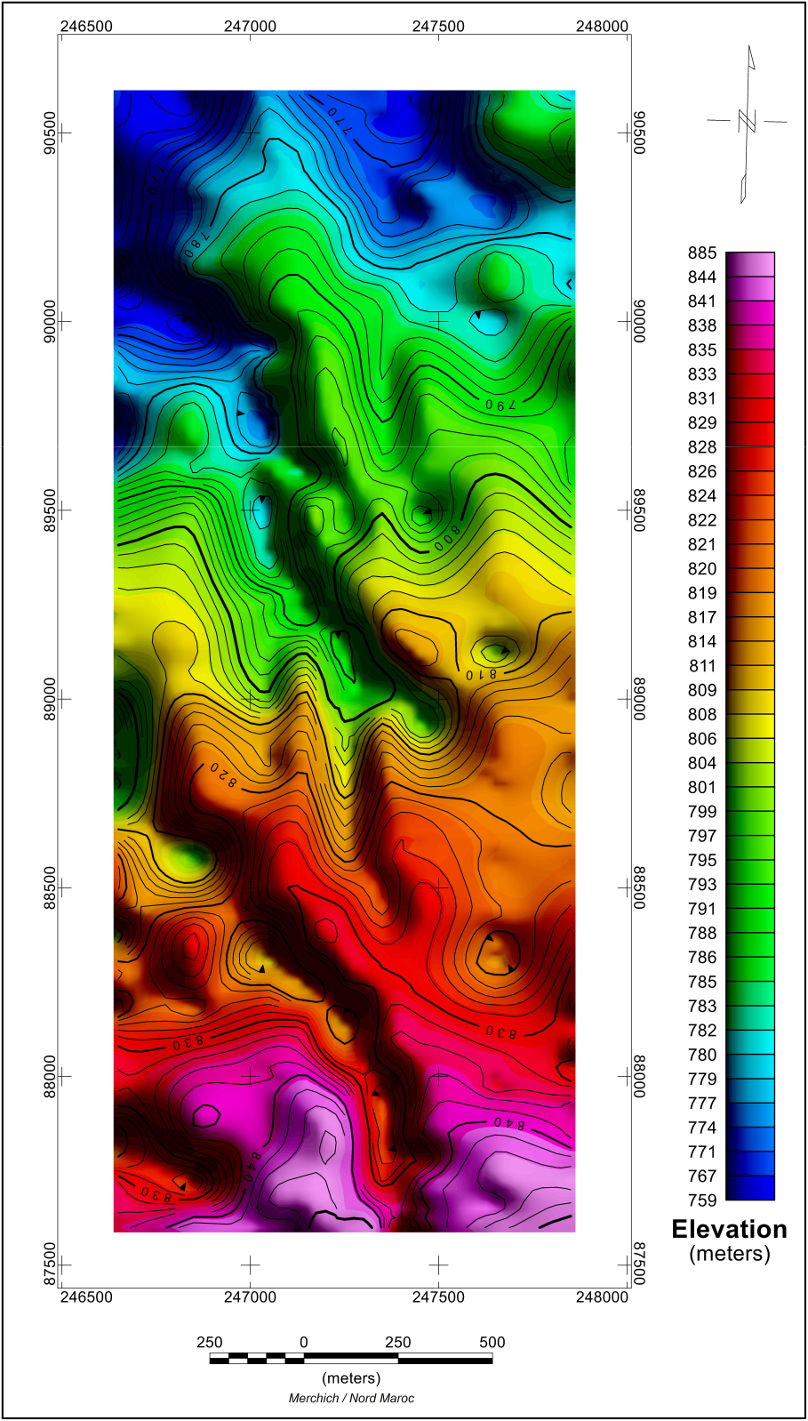
Regional elevation.
See Figure 10.