


 CC-BY 4.0
1. Introduction
Most, if not all, of hydrological models are conceptual models requiring validation tests specific to their desired objective [de Marsily 1994]. When these models are applied under non-stationary conditions e.g. for climate and land use change impact studies, it is necessary to ensure that their structure/parameters are transferable in time [Thirel et al. 2015], by adopting more rigorous cross-validation tests, e.g. the differential split-sample test proposed by Klemeš [1986]. This strategy is rather limited since models are often developed and used for extrapolation. Consequently, pure cross-validation for specific environmental changes is seldom possible, because of a lack of historical environmental conditions similar to projected environmental conditions. An appealing way to circumvent this problem is trading time for space [Peel and Blöschl 2011], the rationale being that if a model can deal with different environments in different locations, it will deal with different environments for different periods at a given location. Despite the widespread use among hydrologists of the “trading time for space” approach [Singh et al. 2011], very few experimental studies were proposed to (in)validate it.
In this paper, we develop a modeling framework designed to test the “trading time for space” method. We start from the simplest expression of rainfall-runoff transformation at the pluriannual time scale using Budyko-type formulations that relate the ratio of long-term average evaporation ratio (E/P) to the ratio of long-term average potential evaporation PET to long-term average rainfall P [Budyko 1974; Ol’Dekop 1911; Schreiber 1904; Turc 1954]. These formulations had perceived a renewed interest over the last two decades since they may provide simple assessment tools to the attribution problem, i.e. they may be employed to separate the effects of climate to other environmental changes on long-term average evapotranspiration and consequently long-term average runoff [Jaramillo et al. 2018; Roderick and Farquhar 2011; Wang 2014]. Adaptations of the classical models flourished intending to include more and more drivers in addition to long-term climate settings [Donohue et al. 2007; Li et al. 2013; Zhang et al. 2004]. Among these attempts, including land use and vegetation characteristics into the model formulation is the most popular since vegetation likely exerts a significant influence on regional water balance and feedback to the atmosphere.
A common feature of the frameworks aiming at developing vegetation-dependent water balance models is to collect hydroclimatic data from climatologically diverse “steady-state” catchments, in the idea to use then these parametrizations for land use changes studies, i.e. trading time for space. The diversity of the catchment set used to derive the parametrized Budyko-type formulations is often put forward as a necessary condition, as advocated by Large-Sample Hydrology groups [Gupta et al. 2014].
Two objectives form the main sections of this article: (i) develop a land use dependent Budyko formulation based on an extensive set of 5026 worldwide catchments to encompass a large variety of climatic and land use conditions, (ii) assess the potentialities of the derived land use dependent Budyko formulation to detect and quantify hydrological impacts of land uses modifications at the catchment scale. As stated by Singh et al. [2011] on climate, the hypothesis is that the spatial relationship between land use and streamflow characteristics is similar to the one observed between land use and streamflow over long periods at a single location.
2. Material
2.1. Data
We selected a large sample of catchments, from several international and national databases: the Global Streamflow Indices and Metadata Archive (GSIM) [Do et al. 2018] consisting of a collection of streamflow time series for more than 35,000 catchments worldwide, the 9322 GAGE-II US stream gauges maintained by the U.S. Geological Survey (USGS) [Falcone 2011], the HydroPortail database (http://www.hydro.eaufrance.fr), where flow measurements are available for more than 4000 stations across France [Leleu et al. 2014] and the UK National River Flow Archive for which streamflow data for more than 1500 stations are available. Since the GSIM database contains catchments from the national databases (France, UK, US) we consider extracting data from these national databases preferable and excluding catchments for these countries from the GSIM database, to avoid any duplicated catchments. The selection was made following two criteria:
- Availability of at least five years of annual streamflow data between 1992 and 2015. This criterion stems from the use of plurennial water balance models and the availability of land use historical data.
- Catchment area between 10 km2 and 10,000 km2. The motivation for the lower limit was due to the spatial resolution of the climate reanalysis data (1/24°), and the upper limit was set so that reduce mixing effects of both land use and climate over a given catchment.
Applying the above criteria led to a selection of 6002 catchments. As many of these catchments are nested within each other, this poses the problem of redundant information that may bias model evaluation using classical cross-validation experiments. To remove redundancy, we subset the database to reach a final set of 5026 non-nested catchments (Figure 1). The catchment represents a large variety of climatic conditions but with a lack of representation of drylands, originating from a lack of river network in these areas. The mean number of available years over the catchment set is 18 and the mean catchment area is 1800 km2. According to the Koppen classification, majority of catchments (64%) are under mild temperate climate, 19% are under snow environment, 12% are under tropical climate and only 3% and 2% are under dry and polar climates respectively.

(a) Location of the 4539 hydrometric stations of the catchment set and mean annual flow over the record period and (b) dominant Koppen climate type distribution of the catchment set.
Climatic data were extracted from the TerraClimate gridded data [Abatzoglou et al. 2018], with a spatial resolution of 1/24°. Annual precipitation (P), Penman–Monteith potential evaporation (PET), and net radiation (Rn) were retrieved for each catchment over the period 1992–2018 and temporally aggregated at an annual time scale. TerraClimate uses climatically aided interpolation, combining high-spatial-resolution climatological normals from the WorldClim dataset, with monthly data from other sources namely CRU Ts4.0 and JRA-55.
Land use data were extracted from the ESA CCI Land Cover time-series [ESA 2017], for which historical land use maps are available at the annual time-scale over the period 1992–2018 at a spatial resolution of 300 m. This dataset was produced in two steps: first, the Medium Resolution Imaging Spectrometer (MERIS) archive from 2003 to 2012 was used to construct a 10-year baseline land cover map, second, the annual time series are obtained by combining the baseline map with land cover changes detected from (i) Advanced Very-High-Resolution Radiometer (AVHRR) time series from 1992 to 1999, (ii) SPOT-Vegetation (SPOT-VGT) time series from 1998 to 2012 and (iii) PROBA-Vegetation (PROBA-V) and Sentinel-3 OLCI (S3 OLCI) time series from 2013 to 2019. The original classification of ESA CCI Land Cover contains 21 classes (Table 1). A 6-level aggregation product was derived using the original classes into IPCC classes that are conventionally used to detect land use change at the global scale. Though highly simplified, this 6-level land use classification appears as a reasonable compromise between the expected role of land use on evaporation and the representativeness of each land use over the catchment set (Figure 2).
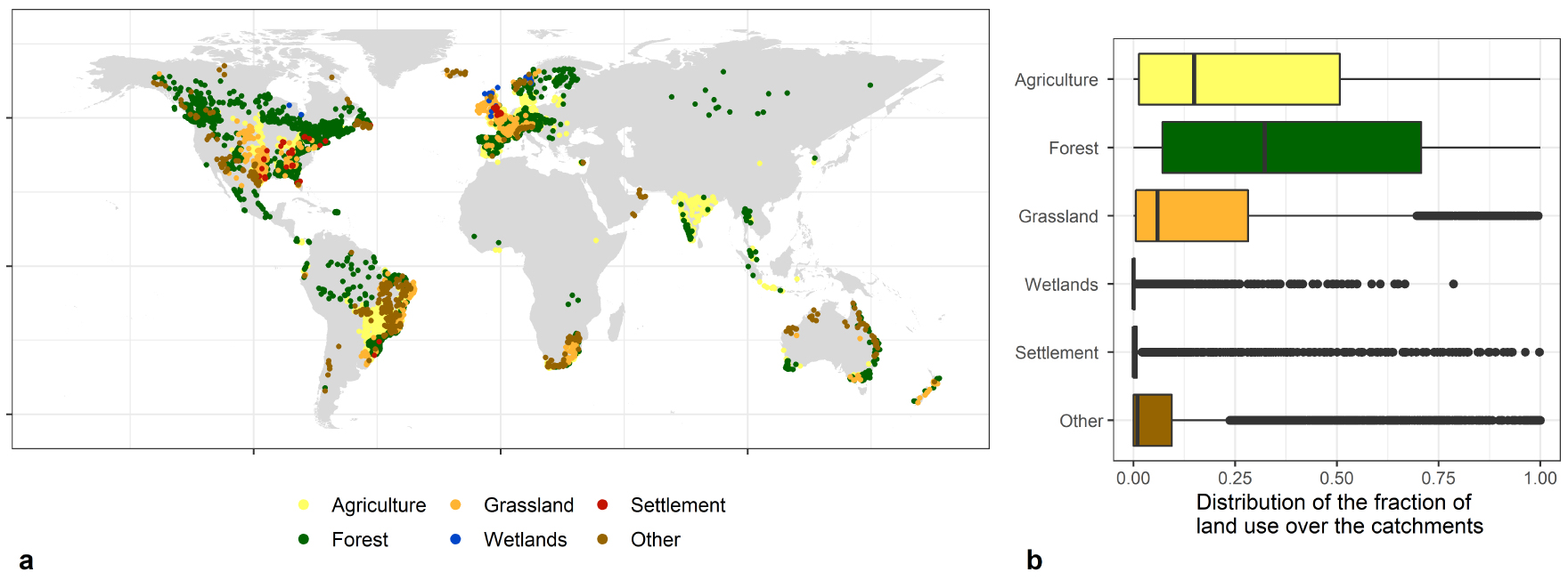
Map of catchments’ (a) dominant land use and (b) distribution of fraction cover for each of the 6 land use classes over the catchment set.
Land use classes considered in this paper
| IPCC classes | Original legend from CCI-LC maps |
|---|---|
| 1. Agriculture | 1. Rainfed cropland |
| 2. Irrigated cropland | |
| 3. Mosaic cropland (dominant) with natural vegetation (tree, shrub, herbaceous cover) | |
| 4. Mosaic natural vegetation (dominant) and cropland | |
| 2. Forest | 5. Tree cover, broadleaved, evergreen |
| 6. Tree cover, broadleaved, deciduous | |
| 7. Tree cover, needle-leaved, evergreen | |
| 8. Tree cover, needle-leaved, deciduous | |
| 9. Tree cover, mixed leaf type (broadleaved and needle-leaved) | |
| 10. Mosaic tree and shrub (dominant) with herbaceous cover | |
| 3. Wetland | 11. Tree cover, flooded, fresh, or brackish water |
| 12. Tree cover, flooded, saline water | |
| 13. Shrub or herbaceous cover, flooded, fresh-saline, or brackish water | |
| 4. Grassland | 14. Mosaic herbaceous cover (dominant)/tree and shrub |
| 15. Grassland | |
| 5. Settlement | 16. Urban |
| 6. Other | 17. Shrubland |
| 18. Lichens and mosses | |
| 19. Sparse vegetation (tree, shrub, herbaceous cover) | |
| 20. Bare areas | |
| 21. Water |
2.2. Tixeront–Fu formulation and benchmark water balance models
Several equations/models were developed under the Budyko framework. In this study, we used the so-called Tixeront–Fu parametrized equation [Fu 1981; Tixeront 1964], which was used in many previous studies [Li et al. 2013; Teuling et al. 2019; Zhang et al. 2004]. This formulation includes one free parameter and we hypothesized in this study that this parameter may depend on land use. Three calibration-free models, namely the Schreiber [1904], the Ol’Dekop [1911] and the Budyko [1974] equations are also used as benchmarks. The equations of these models are presented in Table 2.
Equations of the water balance models used in the study
| Model | Equation | Parameters | Reference | |
|---|---|---|---|---|
| Schreiber |
|
(1) | None | Schreiber [1904] |
| Ol’Dekop |
|
(2) | None | Ol’Dekop [1911] |
| Budyko |
|
(3) | None | Budyko [1974] |
| Tixeront–Fu |
|
(4) | 𝜔 | Tixeront [1964]; Fu [1981]; Zhang et al. [2004] |
P represents the mean annual precipitation, E represents the mean annual evaporation and PET represents the mean annual potential evaporation.
2.3. Tixeront–Fu parameter determination
Li et al. [2013] reviewed numerous studies aiming at determining the parameter 𝜔 of the Tixeront–Fu equation. As an integrator of many physical processes in water and energy budgets, 𝜔 can potentially be related to many physiographic patterns of a catchment: land surface characteristics, including vegetation, soil types, and topography, as well as climate intra-annual variability (e.g. seasonality of P and PET). Given that land use reflects integrated landscape properties, we hypothesized in this study that prescribing a single value of 𝜔 for each land use class might improve the performance of the Tixeront–Fu model. This is done by spatially averaging the contribution of E∕P for each land use class present within each catchment, following (5), and illustrated in Figure 3:
| (5) |
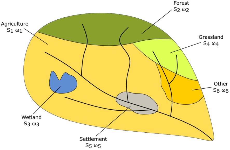
Spatial averaging of the contribution of E∕P for each land use class in the Tixeront–Fu model (5).
Given (5), the number of free parameters is equal to the number of land use classes considered, i.e. six classes. The calibration of these parameters was dealt with a single objective function based on the root mean square error over the catchment set (6) over a range of acceptable values of 𝜔 from unity to five. Below this lower limit, the physical basis of the equation is lost and above the upper limit, the equation is only slightly modified. This objective function is minimized during the calibration process.
| (6) |
| (7) |
2.4. Attributing changes in evaporation rates to climate and land use changes
For each catchment presenting more than 20 years of data (n = 2462), the record period was split into two independent periods (noted “1” and “2”). The change in observed evaporation ratio (𝛥y) between periods 1 and 2 was decomposed into a change related to climatic variability (𝛥yc) between the two periods, and a residual change (𝛥yr) that can be compared to the estimated change due to land use conversions (𝛥yLU):
| (8) |
| (9) |
| (10) |
| (11) |
| (12) |
3. Results
3.1. Catchment water balance analysis under the Budyko framework
In this section, the physical plausibility of the water balance at each catchment is assessed. Three categories of catchments are identified on the Budyko graph and located in Figure 4.
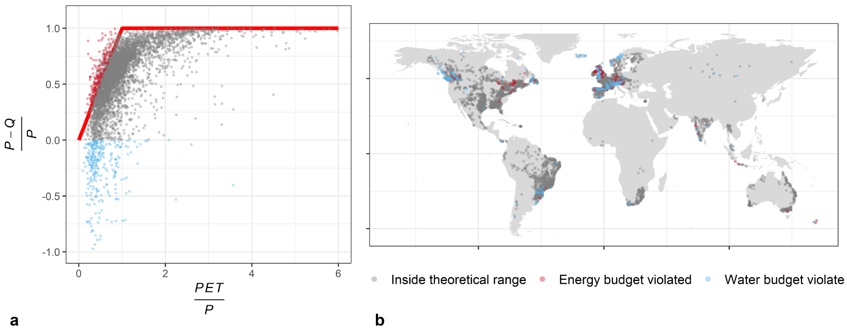
(a) Catchment water balance in the non-dimensional Budyko graph and (b) location of their corresponding hydrometric stations. Catchments where the evaporation ratio is lesser than zero indicate that the mean annual runoff is greater than the mean annual precipitation received by this catchment, hence violating the water budget (blue points), while catchments where latent heat flux exceeds net radiation (red points) violate the energy budget. Note that 31 catchments present evaporative ratio lesser than −1.0 and are not displayed on panel (a). Masquer
(a) Catchment water balance in the non-dimensional Budyko graph and (b) location of their corresponding hydrometric stations. Catchments where the evaporation ratio is lesser than zero indicate that the mean annual runoff is greater than the mean annual precipitation received ... Lire la suite
299 catchments (i.e. 6% of the catchment set) present inconsistent water balance (Q > P). Those catchments are mainly located in high relief contexts (Figure 4) where problems in estimating precipitation (and particularly underestimation of snowfall) accurately are frequent. Other plausible reasons are uncertainties in streamflow estimation, wrong catchment delineation, and/or unknown interbasin groundwater flows. 150 catchments (i.e. 3% of the catchment set) present inconsistent energy balance (E > Rn). Rn was chosen as a more physical limit of E compared to potential evaporation (PET) since analysis on PET might be largely influenced by the formulation used to derive PET. As a comparison, 364 catchments present E larger than Penman–Monteith PET. These catchments are mainly located in humid energy-limited regions, where latent heat flux (or E) are deemed close to net radiation (or PET). Except for this trivial observation, no clear patterns emerged from the location of these catchments since the reasons for violating the energy budget are several, including measurement errors of precipitation, streamflow, or net radiation. The remaining 4538 (i.e. 91% of the initial catchment set) present consistent water and energy balance. Still, these catchments can present other inconsistencies (which remain unknown here), and many of these catchments are close to the theoretical limits in terms of water and energy budget. Since there is no automatic/objective way to investigate the plausibility of water and energy balances on the remaining 4538 catchments, no further investigation was conducted on these catchments and the analyses presented in the forthcoming sections are restricted to those 4538 catchments.
3.2. A land use dependent model using a large sample of catchments
Calibration results indicate relatively similar RMSE values for the different tested water balance models (Table 3). RMSE values range from 0.150 (for the Tixeront–Fu with calibrated 𝜔 specific for 6 land use classes) to 0.181 (for the Ol’Dekop model). Increasing the number of free parameters allows to achieve more satisfying performance, but the calibration of a single parameter for all land use classes only very marginally increases performance compared to the original non-calibrated models. The improvement brought by including land use information is about 0.003 in terms of RMSE (from 0.153 for the Tixeront–Fu model with the same 𝜔 calibrated for all land uses to 0.150 for the Tixeront–Fu model with calibrated 𝜔 specific for 6 land use classes), representing a relative decrease of 2%. The coefficient of determination R2 provides a similar assessment and it increases from 0.544 for the non-calibrated Schreiber model to 0.571 for the Tixeront–Fu model with 6 land use classes.
Calibration results over the entire catchment set
| Model | RMSE | R2 | Number of calibrated parameters |
|---|---|---|---|
| Schreiber [1904] | 0.153 | 0.544 | 0 |
| Ol’Dekop [1911] | 0.181 | 0.561 | 0 |
| Budyko [1974] | 0.158 | 0.557 | 0 |
| Tixeront–Fu with the same 𝜔 calibrated for all land uses | 0.153 | 0.555 | 1 |
| Tixeront–Fu with calibrated 𝜔 specific for 6 land use classes | 0.150 | 0.571 | 6 |
The differences in terms of prediction of the evaporative ratios are quite small but visible when analyzing the correlation between observed and simulated evaporative ratios (Figure 5). The analysis of the residuals of the Tixeront–Fu model with calibrated 𝜔 specific for 6 land use classes does not allow identifying some specific conditions for which the model fails (Figure 6). The model appears less efficient on small catchments compared to large catchments and it also encounters difficulties in cold regions. The distributions of the residuals are relatively homogenous along with land use classes. Catchments where wetlands are dominant, are poorly modeled but these catchments are very few (n = 10).
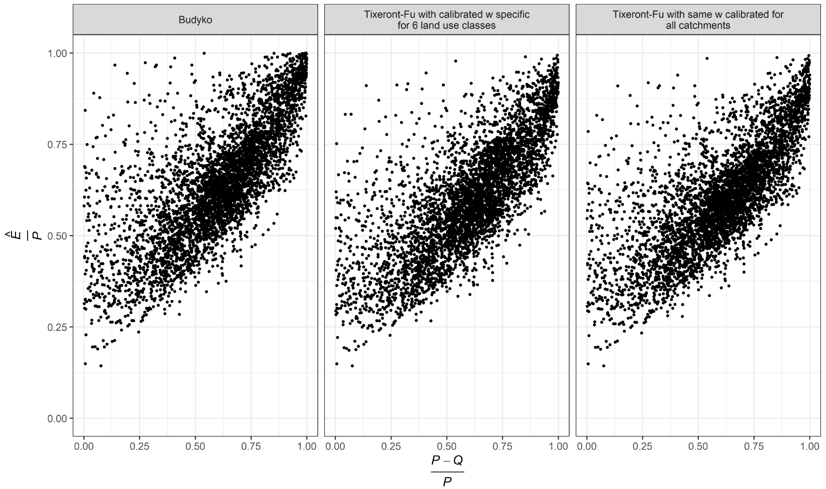
Observed and simulated evaporative ratios by three different models with zero to six calibrated parameters. Results are shown in calibration mode.
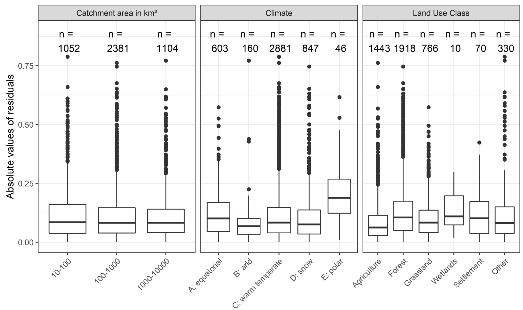
Residuals of the Tixeront–Fu model with calibrated 𝜔 specific for 6 land use classes. The distributions of the absolute values of the residuals are represented by boxplots according to the characteristics of the catchment in terms of drainage area, climate class, and dominant land use class. The lower and upper hinges correspond to the first and third quartiles and the upper and lower whiskers extend from the hinge to the largest value no further than 1.5 ∗ IQR from the hinge (where IQR is the interquartile range). Masquer
Residuals of the Tixeront–Fu model with calibrated 𝜔 specific for 6 land use classes. The distributions of the absolute values of the residuals are represented by boxplots according to the characteristics of the catchment in terms of drainage area, climate ... Lire la suite
For all models, the RMSE obtained in validation are quite similar to those obtained in calibration (Figure 7), showing that the models are spatially robust, i.e., the spatial transferability of the model parameters is satisfying. This is reassuring and confirms that the dataset is broad enough to draw stable and significant conclusions. In validation, the advantage of a parameter-specific land use classification remains.
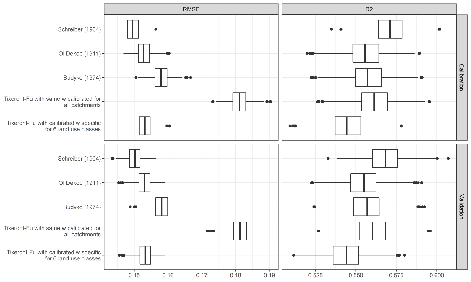
Cross-validation results for the three benchmark models and the two calibrated Tixeront–Fu models. The boxplots represent the distribution of the two assessment criteria (RMSE and R2) for the 500 realizations of the split sample test. The lower and upper hinges correspond to the first and third quartiles and the upper and lower whiskers extend from the hinge to the largest value no further than 1.5 ∗ IQR from the hinge (where IQR is the interquartile range).
The parameter values obtained by calibrating the Tixeront–Fu model equation with 6 different land use classes are rather spread over the range of possible values, from close to unity to 5 (Figure 8), and relatively consistent with a priori expectations. The “Settlement” land use class reaches a low median parameter value of 1.78 (interquartile range: 1.72–1.83) indicating low evaporation ratios, while flooded vegetation gets a median parameter value of 5.00 (interquartile range: 3.54–5.00), indicating evaporation close to potential evaporation, which is physically consistent given that water is not a limiting factor on these landscapes. Forest and grassland show close parameter values, with median values at 2.08 and 2.11 and interquartile ranges of 2.06–2.10 and 2.09–2.14, respectively. Among the most common land use, agriculture gets a remarkably high parameter value, with a median at 2.81 (interquartile range: 2.79–2.84). The large range of parameter values for the land use class “Other” is probably explained by the large diversity of land use composing this class, and their diverse behavior relative to evaporation (e.g. sparse vegetation, shrublands, bare areas, see Table 1). As a consequence, the median parameter value is close to the optimal lumped value, with a median at 2.33 (interquartile range 2.27–2.43).
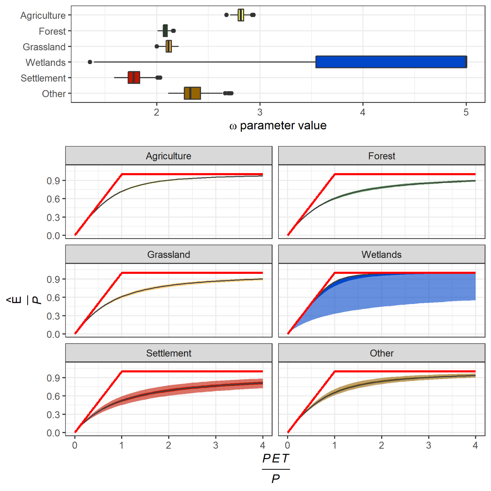
𝜔 parameter values for 6 land use classes (upper). The boxplots represent the distribution of the 500 split-sample tests. The lower and upper hinges correspond to the first and third quartiles and the upper and lower whiskers extend from the hinge to the largest value no further than 1.5 ∗ IQR from the hinge (where IQR is the interquartile range). Corresponding Budyko curves (lower) with predictive bounds, based on the interquartile ranges.
3.3. Trading space for time: analyzing model behavior on transient catchments
In this section, we assess the ability of the Tixeront–Fu model equation with 6 different land use classes to predict the effect of land use changes on evaporation ratios. To do so, we compared the change in evaporative ratio due to land use (12), to the residual change in evaporative ratio computed as the difference between the total change, and the change due to climate variations across the two subperiods (10).
For many catchments, the Tixeront–Fu model parametrized to take into account explicitly land use typology fails to predict change in evaporative ratio due to land use change (Figure 9). Generally speaking, the estimated change is quite small compared to the observed change, meaning either that the model inappropriately reproduces the role of land use on evaporative ratios or that the observed change is due to factors other than climate and land use.
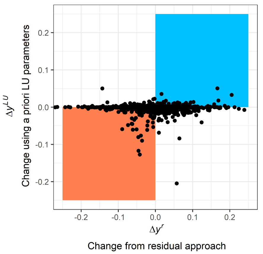
Observed and simulated changes in evaporative ratios as estimated by the residual approach and the Tixeront–Fu model with 6 different land use classes. Dots located in blue and red rectangles correspond to catchments for which the evaporative trend sign is correctly predicted either positive or negative, respectively.
To address more specifically the former hypothesis, we restrict our analysis to those catchments that experienced important gross land use change. Three typical land use conversions are considered: (i) the conversion from forest to arable land, to constitute this sample, we retained the catchments for which the fraction of arable land increased up to 0.1 while the fractions of forest decreased up to 0.1; (ii) the conversion from arable land to forest, to constitute this sample, we retained the catchments for which the fraction of forest increased up to 0.1 while the fractions of arable lands decreased up to 0.1; (iii) the conversion of vegetated lands to urban areas, to constitute this sample, we retained the catchments for which the fraction of urban area increased up to 0.1 while the fractions of other vegetated areas (forest, arable and grasslands) decreased up to 0.1. This leads to the selection of 52 catchments: 27 urbanizing, 10 from agriculture to forest, and 15 from forest to agriculture.
Since the selected catchments are indeed experiencing important land use change, the simulated change of evaporative ratio is more visible (Figure 10) than when considering the whole catchment set. However, the model still fails to detect the sign and intensity of change for the conversion from arable land to forest and vice-versa. Urbanization is the sole type of conversion for which the model can reproduce the effect on evaporative ratio, with a decreasing trend of evaporation with urbanization.
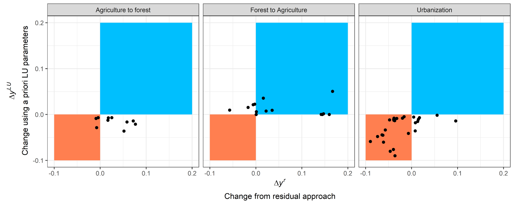
Observed and simulated changes in evaporative ratios as estimated by the residual approach and the Tixeront–Fu model with 6 different land use classes for three types of land use changes. Dots located in blue and red rectangles correspond to catchments for which the evaporative trend sign is correctly predicted either positive or negative, respectively.
4. Discussion
4.1. Comparison with previous model parametrization and performance
Before comparing the modeling results of this study with previous attempts, it is important to keep in mind that such comparison is complex due to (i) the relatively small number of large sample studies, (ii) the different target variables within these studies, and (iii) the different data prefiltering methods. We found that 449 catchments (9% of the total catchment sample) did not fall within the theoretical range for the evaporative ratio. This ratio is similar to previous studies on the global scale: Peel et al. [2010] and Zhou et al. [2015] found ratios of 19% and 10% for global streamflow datasets constituted by 861 and 1928 worldwide catchments, respectively. The choice of including these catchments or not for developing and assessing a hydrological model is not trivial. On the one hand, including these catchments may lead to greater uncertainties in the estimations of model parameters value but on the other hand, excluding these catchments poses the question of the validity of the remaining catchments, that are still susceptible to have water balance issues. For these reasons, some authors included further data checks, including assessments of the impacts of dams or preliminary estimation of interbasin groundwater flows [de Lavenne and Andreassian 2018], which may affect significantly water balance for some geological settings.
This choice also has important consequences on the performance of the model since water balance formulations from the Budyko framework are not able to reproduce the behaviors of the catchment that do not fall within the theoretical range. As a consequence, studies that prefilter hydroclimatic data before assessing model performance show remarkably better modeling results than those without or with basic filtering (Table 4). Probably the most similar study in terms of data is the study by Beck et al. [2015] who developed dedicated neural networks for a set of flow characteristics including mean annual runoff (QMEAN) and runoff yield (i.e. QMEAN/PMEAN). To compare our results with previous studies, we compute additional performance metrics, including R2 and RMSE on several mean annual variables. The obtained performance metrics are very similar to those obtained by Beck et al. [2015] with a very different modeling approach (Table 4).
Comparison of model performance with previous studies
| Reference | This study | This study | Beck et al. [2015] | de Lavenne and Andreassian [2018] | Oudin et al. [2008] | Sanford and Selnick [2013] |
|---|---|---|---|---|---|---|
| Modeling approach | Tixeront–Fu model with fixed w | Optimized model with 6 parameters | Neural network | Tixeront–Fu model including a seasonality index | Parametrized Budyko model | Climate-based regression |
| Number of catchments | 4539 | 4539 | 4079 | 171 | 1508 | 838 |
| Filtering of data | Basic | Basic | Basic | Advanced | Advanced | Basic |
| Spatial scale | Global | Global | Global | France | Global (but mainly France, US and UK) | US |
| RMSE (y) | 0.153 | 0.150 | 0.051 | 0.052 | ||
| RMSE (QMEAN) (mm/yr) | 172.1 | 169.6 | 51.4 | 52.9 | ||
| RMSE (sqrtQ) | 3.87 | 3.82 | 3.91 | |||
| R2 (ET_MEAN) | 0.611 | 0.621 | 0.882 | |||
| R2 (sqrtQ) | 0.800 | 0.804 | 0.88 |
4.2. Is the role of land use significant and relevant?
As stated in Section 3.2, the improvement brought by incorporating specific 𝜔 parameter value for each land use is modest: RMSE on evaporative ratio-y varied from 0.153 for the Tixeront–Fu model with the same 𝜔 calibrated for all land uses to 0.150 for the Tixeront–Fu model with calibrated 𝜔 specific for 6 land use classes. Previous attempts to improve Budyko formulations by adding free parameters also report marginal improvements: Oudin et al. [2008] improved RMSE on the evaporative ratio of 0.007 by including vegetation parameters while de Lavenne and Andreassian [2018] got an improvement of 0.006 by including a seasonality parameter. Considering the much larger and diverse catchment set of the present study, we may consider that the improvement of model performance agrees with previous studies and pointed out the difficulty to improve Budyko-type formulations. One may argue that the modest improvement might come from the fact that land use is not as important as expected in explaining catchment-scale water budgets. From the literature results, it is not clear whether the Tixeront–Fu parameter shall be related only to land use (and particularly vegetation types) or also to other physiographic and/or climatic characteristics. Previous attempts to regionalize 𝜔 leads to some contrasting results: while Li et al. [2013] found that 𝜔 may be closely related to vegetation coverage, Xu et al. [2013] noticed that the variance of 𝜔 explained by vegetation indices (namely the NDVI) seems low and Abatzoglou and Ficklin [2017] found that vegetation metrics did not improve the determination of 𝜔 compared to some other descriptors such as the ratio of soil water holding capacity to precipitation and topographic slope.
While modest, the improvement of the model performance obtained in Section 3.2 appears significant: a Welch Two Sample t-test on RMSE distributions of the Tixeront–Fu model with the same 𝜔 calibrated for all land uses and the Tixeront–Fu model with calibrated 𝜔 specific for 6 land use classes leads to a p-value below 0.005. Therefore, interpreting the parameter values for each land use class makes sense. The 𝜔 parameter values obtained in this study can be compared in range and in order with previous studies (Table 5). Investigating the 𝜔 parameter of the Tixeront–Fu water balance model on a selection of lysimeter data, Teuling et al. [2019] found for settlement the value of 1.3, for grassland/cropland 1.7, while forest presents the larger value. Zhang et al. [2004] differentiated two land use: grassland and forest with values of 2.55 and 2.84, respectively. The comparison of absolute values is biased by methodology, including the choice of the potential evaporation equation or the way to determine the parameter values, but it appears that 𝜔 parameter values are inconsistent in terms of relative values for forest, grassland, and cropland: the value we obtained for agriculture and forest are particularly high and low respectively, compared to these previous studies. Interestingly, Williams et al. [2012] using a synthesis of evapotranspiration measured across a global network of flux towers also found that grasslands and croplands have on average a higher evaporative ratio than forested landscapes, which tends to corroborate our findings.
𝜔 parameter values for several land use classes given by the present study and two other studies
| Data and methods | This study | Zhang et al. [2004] | Teuling et al. [2019] |
|---|---|---|---|
| Catchment scale with fractional land use | Catchment scale with dominant land use | Lysimeter data | |
| 𝜔 for agriculture | 2.81 (IQ range: 2.79–2.84) | 1.7 | |
| 𝜔 for forest | 2.08 (IQ range: 2.06–2.10) | 2.84 | [2.3–3.1] |
| 𝜔 for grassland | 2.11 (IQ range : 2.09–2.14) | 2.55 | 1.7 |
| 𝜔 for wetlands | 5.00 (IQ range: 3.54–5.00) | ||
| 𝜔 for settlement | 1.78 (IQ range 1.72–1.83) | 1.3 | |
| 𝜔 for other | 2.33 (IQ range 2.27–2.43) |
Note that Teuling et al. [2019] used a rather different PE equation and acknowledged that this may lead to lower 𝜔 values.
4.3. Why trading space for time is inefficient?
The land use dependent model developed in this study appears inappropriate to describe the change in time of the evaporative ratio of the majority of catchments, even for those catchments that experienced important land use change. This is not good news for hydrologists who are asked to develop models able to integrate climate and land use scenarios, to help water resources planning and management [Milly et al. 2008]. In our opinion, this relative failure may be due to either the over-simplistic Budyko framework, or the fact that land use loses its interest when trading space for time. These points are discussed hereafter.
While the use of the Budyko framework is advocated by many authors for attribution studies [Wang and Hejazi 2011], its crudeness may not allow it to model land use change effect on evapotranspiration. To fit the simplicity of the Budyko framework, we designed in this paper a semi-lumped approach by combining the responses of the diverse land use fractions in a catchment. We hypothesized that the hydrological behavior of a land use class may be formulated by adjusting a single parameter of the Tixeront–Fu model by considering that this behavior for each land use class is homogenous across environmental conditions. This is probably a too crude assumption but a more detailed description of the soil-vegetation-atmosphere hydrological processes would come with heavier parametrization. Indeed, the idea that assessing land use changes can only be made through distributed model with physical bases is well-spread in literature [Beven 2002; Wijesekara et al. 2012].
The pluriannual time step makes it impossible to integrate the seasonality effects of climate and vegetation activity. Some studies intend to parametrize the climate seasonality effect [de Lavenne and Andreassian 2018; Potter and Zhang 2009], but the seasonal patterns of vegetation transpiration might also be taken into account within these parametrizations, as perennial vegetation generally transpires throughout the spring, summer, and autumn seasons, while the majority of the transpiration from crops occurs during the summer.
In contrast with the one-parametrized model, the effects of vegetation change can be subtle and the impacts of some major land use changes are still subject to debate [Andréassian 2004; Beck et al. 2013]. Land use changes might also influence water balance only until a long time period so that the new vegetation cover reaches maturity [Kuczera 1987]. Wang [2014] proposed to distinguish two types of human-induced changes: the changes that yield measurable effect on water balance just after the activity is in places such as surface water abstraction/diversion and storage, and the changes that yield measurable effect only until a long time period. Our results suggest that urbanization may belong to the latter since its impact on the evaporative ratios is relatively well detected and quantified by the model proposed in this study. Conversely, vegetation changes may belong to the former type of changes, with highly case-specific changes.
Finally, the space for time trading concept presents inherent caveats [Berghuijs and Woods 2016] due to the non-orthogonality of climate, land use, and other physiographic descriptors such as topography, and soil types [Troch et al. 2015; van Dijk et al. 2012; Xu et al. 2013]. As perennial vegetation may be viewed in equilibrium with environmental conditions, the spatially calibrated model parameters are likely related to other factors like vegetation, e.g. water holding capacity, slope. When applied to non-stationary conditions, vegetation covers may change while the other characteristics remain, at least for some time, which may explain to a certain extent the failure of the model under non-stationary conditions.
5. Conclusion
Empirical assessments of the impact of land use on water balance are not straightforward. While the Budyko framework is often advocated as a simple but efficient way to distinguish the effects of climate and land use on water balance, very few studies applied it on large samples of non-stationary catchments. In this paper, we adapted the Budyko framework to develop a land use dependent water balance model using a large sample of 4539 catchments worldwide and we then applied it under non-stationary conditions, by trading time for space. Despite slight but significant improvements of the model to differentiate the role of several land use across catchments, the model fails to predict both the sign and the magnitude of change in evaporative ratios due to land use changes, except the case of urbanization. In 1994, de Marsily pointed out that the constraints of Greek tragedy (uniqueness of place, time, and action) applied to empirical hydrological models. Even with the progress in model developments and availability of worldwide hydro-climatic data, we shall acknowledge that de Marsily’s view is still relevant.
Conflicts of interest
Authors have no conflict of interest to declare.
Acknowledgements
This study utilized data from several sources. For streamflow data and catchment delineation, we used GSIM database (https://doi.pangaea.de/10.1594/PANGAEA.887477) that makes available data from a large number of worldwide catchments. For the U.S. catchments, streamflow data were collected from the USGS website (available at http://waterdata.usgs.gov/). For the French catchments, flow measurements were extracted from HydroPortail (available at https://www.hydro.eaufrance.fr/). For the UK catchments, streamflow and contours data were collected from the National River Flow Archive (https://nrfa.ceh.ac.uk/data/). Precipitation and potential evaporation data were obtained from the TerraClimate database (available at https://www.climatologylab.org/terraclimate.html). We thank Antoine Carlier for his help on Figure 3, the invited editors to provide us the opportunity to contribute to this special issue, Thibault Mathevet and the anonymous reviewer for their relevant suggestions.