


 CC-BY 4.0
1. Introduction
In four decades on inverse problem in hydrogeology, de Marsily et al. [2000, see also de Marsily et al. 1999] observe that “in hydrogeology, there are a great number of competing methods for solving the inverse problem”. Kitanidis [1995] notes: “although the consensus is that the linear method is appropriate only when the variance of log conductivity is less than 1, in my experience the method may work reliably for larger variances provided that the variation happens to be gradual or in the direction perpendicular to the streamlines”. However, referring to the comparison of methods for solving the inverse problem carried out by several teams on four synthetic data sets, Zimmerman et al. [1998] point out “the evident superiority of the nonlinear methods as compared with linear ones”. In a more recent review of the inverse problem, Illman [2014] presents the evolution of approaches for mapping heterogeneity.
In this paper, we come back to the early cokriging of the transmissivity from transmissivity and head measurements, based on the linearisation of the flow equation linking head and transmissivity fluctuations. First a non-exhaustive historical review of geostatistical modelling based on the linearisation of flow equations is given. The relationships between simple and cross-covariances of transmissivity and head fluctuations for two quasi-steady state flows established by Zhang and Neuman [1996] in another context are applied to the inverse problem. On synthetic cases original results show the interest of crossing two quasi-steady-state flows to improve the estimation of transmissivity. The restrictive hypotheses used for the linearisation of the flow equation are then discussed, as well as the practical application of cokriging of log-transmissivity.
The present paper does not give an extensive review of “geostatistical inversion”, even for methods based on the linearisation of the flow equation. For a substantiated analysis of the difficulties posed by the spatial variability or the heterogeneity of subsurface reservoir properties for flow and transport modelling, the reader is invited to refer to de Marsily et al. [2005]. Neuman’s feedback [2020] also states the importance of spatial variability of parameters. A recent non-exhaustive review of methods for constraining geostatistical estimation by flow physics can be found among others in de Fouquet et al. [2023].
2. Steady state linear flow
2.1. Linearisation of the flow equations
For steady state flow without recharge, the diffusivity equations in two dimensions is written
| (1) |
Delhomme and de Marsily [2005] observe that Equation (1) can be written
| (2) |
Let now x = (x1,x2) denote a point in the plane. In the simplified case with a macroscopic head oriented in the direction with constant modulus J, and constant scalar transmissivity T(x) = T0, the hydraulic head h is linear:
For a transmissivity field with spatial variability, for example when the transmissivity is lognormal T(x) = T0e𝛩(x), let us denote 𝛷 the associated head perturbation: H(x) = h(x) +𝛷 (x).
When only the first order perturbations are retained, Equation (1) becomes:
| (3) |
The initial models of Mizell et al. [1982] and Kitanidis and Vomvoris [1983] linking the covariances of the perturbations 𝛩 and 𝛷 were based on stationarity assumptions. Dagan [1985] calculated a second-order approximation of the covariance of the hydraulic head, observing that “the first-order approximation is very robust and even for a log-conductivity variance equal to unity, the second-order correction of the head variances is smaller than 10% of the first-order approximation”.
Dong [1990] wrote the solution of Equation (3) as follows, since transmissivity cannot generally be assumed to be differentiable:
| (4) |
Matheron also showed that if Z is an IRF-1, the solution 𝛷 of the partial differential equation
The generalised simple and cross covariances between transmissivity and head perturbations which are solution of Equation (4) verify the following relationships, with h = (h1,h2):
| (5) |
The simple (generalised) covariances are even. The cross-covariance is odd, and thus equal to zero for h = 0. The anisotropic variogram of the head perturbation is generally unbounded.
Dong [1989, 1990] and Roth [1995] give the explicit expressions of the generalised covariance of head perturbations as well as the cross-covariance between transmissivity and head perturbations, for usual various models of the variogram of transmissivity. These expressions allow an estimate of the head consistent with Equation (4). Above all they allow estimating transmissivity by co-kriging from head and transmissivity measurements, providing a linearised approximation of the solution of the inverse problem.
In this model, boundary conditions (fixed head, zero flow) are rejected to infinity and occur via the macroscopic gradient of the head. In the cokriging these conditions are introduced as data only at the locations where they are known, and not necessarily all around the modelled field.
The literature presents several applications of this cokriging for solving the inverse problem. Rubin and Dagan [1987] consider that the spatial simple and cross covariances of transmissivity and head depend on a parameter vector 𝜃 which cannot be determined with certainty from the data. They develop the analytical expressions for the conditional covariances when 𝜃 is determined by a maximum likelihood procedure.
Ahmed and de Marsily [1993] perform the cokriging with an approximated but consistent model (ensuring the positivity of variances) of the simple and cross-covariances of head and transmissivity, calibrated to the sample simple and cross-covariances. On a synthetic case approaching a real one, they show that cokriging improves transmissivity estimation compared with kriging. Taking into account the local head gradient rather than the regional one improves the estimation of the transmissivity.
Hernandez et al. [2003] confirm that geostatistical inversion by co-kriging hydraulic head and log-conductivity improves predictions of head and flux compared with conditioning on conductivity or head data alone.
Moreover the expressions (5) of simple and cross covariances between transmissivity and head perturbations can be used for the direct geostatistical simulation of transmissivity, head and flow when linearisation assumptions are valid [de Fouquet 2000; Mariotti et al. 2000].
2.2. Case of two flows
Zhang and Neuman [1996] observed that “even locally uniform gradients tend to show seasonal fluctuations in magnitude and direction”. An example is given in Verley et al. [2003] for the nappe de la Beauce, locally.
Zhang and Neuman examine the effects, on the longitudinal and transverse dispersion respectively, of these temporal fluctuations in the magnitude and direction of the mean velocity by developing the auto and cross-covariances of velocity, head and log conductivity. The previous first-order approach is generalised considering quasi steady-state flow at two times. These expressions of auto and cross covariances of head and log conductivity can also be used for geostatistical inversion by “crossing” two flows, in order to improve the estimation of transmissivity.
Let us revisit their developments. Two macroscopically linear flows, indexed by 1 and 2, are first considered in the same transmissivity field, following two orthogonal directions Ox1 and Ox2. To simplify the presentation, the module J of the macroscopic gradient is assumed to be the same in the two cases. However this hypothesis can be relaxed. Based on the relationships (4), the solutions 𝛷i are written:
| (6) |
| (7) |
For a flow with the same macroscopic head gradient J and any angle 𝛼 with the first coordinate axe, the head perturbation is deduced from the linearity of Equation (6), putting
| (8) |
However it is simpler to choose a base such that . Denoting 𝛽 the angle between the two macroscopic flows, the expressions of the simple and cross covariances are simplified:
| (9) |
Always because of the linearity of the equations, the head of a third flow is expressed as a linear combination of the first two. The co-kriging system with head data from three flows is therefore singular, unless measurement errors are introduced in the variogram of the head data, typically via nugget effects.
3. Example: comparison of cokriging the transmissivity from one or two flows
3.1. Construction of synthetic cases
Cokriging tests are classically performed as follows: (i) geostatistical simulation of a transmissivity field; (ii) flow calculation on this field (using a flow simulator, here Visual Modflow), the fixed macroscopic gradient is imposed via conditions on the boundaries of a larger field; (iii) data extraction far enough from these boundaries; (iv) kriging and cokriging with data from one or two flows.
Several areas are specified (Figure 1):
- the transmissivity is simulated on a “simulated area” of 1600 m × 1600 m;
- the “study area” is 500 m × 500 m from which the data are taken.
The first zone is large enough to fix the boundaries conditions of the various flows. These boundaries conditions define an “intermediate area” of 1100 m × 1100 m, in which the heads are calculated. However, in order for the head data to be far enough from the boundaries, the “study area” is smaller than the “intermediate area” (Figure 1).
Definition of the three areas: simulated area for transmissivity simulation, intermediate area for setting boundary conditions, and study area. The arrow indicates the main flow direction for the represented boundary conditions.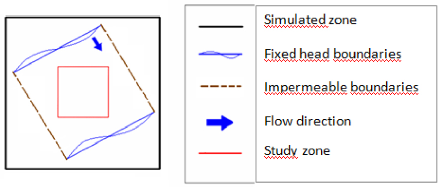
The log-transmissivity is simulated with a spherical variogram with a range equal to 70 m and a sill of 0.5. Three flows with a macroscopic gradient with unit module are calculated
- North to South (NS)
- Northwest to Southeast (NW–SE)
- West to East (W–E)
Initial tests have shown that isolated head data reduce only slightly the estimation variance of transmissivity, while in the vicinity of two close head data, this estimation variance decreases significantly. This is consistent with the known observation that “head variations due to heterogeneity are small, whereas those of velocities and travel time are large” [Matheron and de Marsily 1980].
The co-kriging by two flows is therefore examined with a significant number of close head data (20), cf. Figure 2.
Location of the transmissivity (+) and head (∙) data.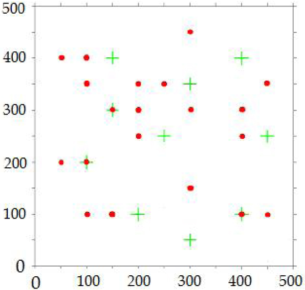
The different estimations of transmissivity are compared according to the following four criteria, where N denotes the number of meshes
- the mean absolute error MAE:
- the mean absolute standardised error MASE:
- the root-mean-square error RMSE:
- and the root-mean-square standardised error RMSSE:
where (log(T))∗ denotes the estimate of log(T) and 𝜎K the standard deviation of the estimation (kriging or cokriging) error. The RMSSE criterion based on the standardised error allow verifying the expected improvement of accuracy by cokriging.
3.2. Comparison between one and two flows
The values in Tables 1 and 2 are given on the decimal logarithm.
Estimation of log-transmissivity on the 500 m × 500 m study area (2601 meshes)
| MAE | MASE | RMSE | RMSSE | ||
|---|---|---|---|---|---|
| Kriging | 0.238 | 0.760 | 0.306 | 0.971 | |
| Cokriging 1 flow | N–S | 0.223 | 0.760 | 0.288 | 0.970 |
| NW–SE | 0.220 | 0.754 | 0.286 | 0.967 | |
| W–E | 0.223 | 0.766 | 0.290 | 0.983 | |
| Cokriging 2 flows | N–S; NW–SE | 0.218 | 0.805 | 0.285 | 1.034 |
| N–S; W–E | 0.214 | 0.790 | 0.281 | 1.015 | |
| NW–SE; W–E | 0.218 | 0.804 | 0.284 | 1.028 |
Values are given on the decimal logarithm.
Estimation of the log-transmissivity in the heterogeneous case, (a) in the local area (121 meshes), (b) on the extended area (961 meshes) and (c) in the study area
| (a) Local area 100 m × 100 m | |||||
|---|---|---|---|---|---|
| MAE | MASE | RMSE | RMSSE | ||
| Kriging | 0.916 | 2.667 | 1.077 | 3.138 | |
| Cokriging 1 flow | N–S | 0.703 | 2.434 | 0.870 | 3.013 |
| NW–SE | 0.612 | 2.184 | 0.758 | 2.716 | |
| W–E | 0.365 | 1.281 | 0.450 | 1.576 | |
| Cokriging 2 flows | N–S; NW–SE | 0.347 | 1.486 | 0.416 | 1.781 |
| N–S; W–E | 0.305 | 1.296 | 0.374 | 1.579 | |
| NW–SE; W–E | 0.326 | 1.393 | 0.406 | 1.747 | |
| (b) Extended area 300 m × 300 m | |||||
| Kriging | 0.300 | 0.905 | 0.462 | 1.372 | |
| Cokriging 1 flow | N–S | 0.317 | 1.079 | 0.436 | 1.494 |
| NW–SE | 0.289 | 0.986 | 0.393 | 1.358 | |
| W–E | 0.260 | 0.879 | 0.336 | 1.134 | |
| Cokriging 2 flows | N–S; NW–SE | 0.319 | 1.211 | 0.398 | 1.513 |
| N–S; W–E | 0.316 | 1.193 | 0.408 | 1.532 | |
| NW–SE; W–E | 0.247 | 0.938 | 0.321 | 1.225 | |
| (c) Study area 500 m × 500 m | |||||
| Kriging | 0.274 | 0.809 | 0.379 | 1.114 | |
| Cokriging 1 flow | N–S | 0.301 | 0.964 | 0.390 | 1.264 |
| NW–SE | 0.270 | 0.871 | 0.351 | 1.149 | |
| W–E | 0.247 | 0.794 | 0.314 | 1.013 | |
| Cokriging 2 flows | N–S; NW–SE | 0.317 | 1.114 | 0.400 | 1.417 |
| N–S; W–E | 0.301 | 1.059 | 0.382 | 1.352 | |
| NW–SE; W–E | 0.239 | 0.840 | 0.305 | 1.078 | |
Values correspond to decimal logarithm.
The mean deviation MAE and the RMSE show that cokriging improves the estimation accuracy of transmissivity compared with kriging, and even more when crossing two flows. However, the standardised deviations are rather stable between kriging and cokriging with one flow, and slightly increase for two-flows cokriging. The RMSSE are close to unity, which shows that the uncertainty is correctly quantified, and somewhat overestimated by kriging or cokriging with one flow.
3.3. Detection of a transmissivity barrier
The second test field presents a low transmissivity barrier of 10−6 m2⋅s−1 compared to a previous average value of 10−4 m2⋅s−1. The variogram model of transmissivity remains unchanged, because no transmissivity data is located in the barrier.
The test is performed with only four transmissivity data. The quality criteria are first calculated on a small area of 100 m × 100 m, centred on the anomaly (Figure 3), in order to verify if cokriging helps detect the heterogeneity.
Location of the heterogeneity, represented by an ellipse. Central square: local area; dashed square: extended area.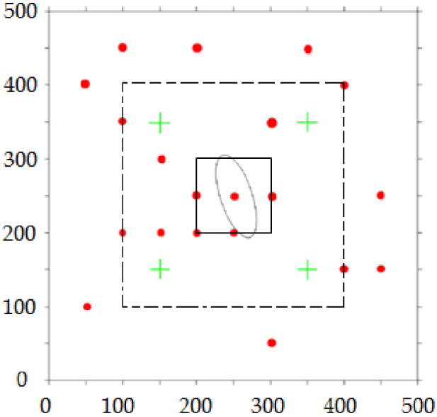
The MAE and the RMSE (Table 2a) show that the N–S or NW–SE flows, which are yet little impacted by the transmissivity barrier, improve the estimation. Logically the W–E flow, which crosses the barrier, informs the best on the transmissivity field: the mean deviation MAE and the RMSE decrease by almost 60%. Note that, with a mean deviation of 0.347, the combination of the N–S and NW–SE flows gives an estimation accuracy comparable to that of the W–E flow, with a mean deviation of 0.365. The lowest errors (MAE, RMSE) are obtained by cokriging using the N–S and W–E flows, which both cross the barrier.
The standardised deviations are large: the method allows detecting the heterogeneity, but with only four transmissivity data located outside it, the estimation accuracy remains poor. However, the increase in the variance of the transmissivity field was not taken into account in the modelling.
These results are consistent with Kitanidis remark [1995] cited in the introduction according to which “the method may work reliably […] provided that the variation happens […] in the direction perpendicular to the streamlines”.
The results are less satisfactory on a larger scale. In the extended area of 300 m × 300 m, bounded by dashes lines on the figure, the head data improve or on the contrary deteriorate the MAE, depending on the configurations, but in all cases the RMSE decreases compared with kriging. The estimations are poorly improved by the head data of the N–S flow, which is visible on the estimation maps (Figure 4): the low transmissivity barrier is detected, but the surrounding area shows large transmissivities that do not exist. Once again, the head data from the W–E flow improve greatly the precision, and to a lesser extent, it is the same for the NW–SE flow. The MAE and RMSE criteria are minimal when crossing these two flows (Table 2b). In all cases, the RMSSE remains greater than one, for the same reason as on the local area.
Decimal logarithm of Transmissivity field. (a) Estimation from N–S flow; (b) estimation from NW–SE flow; (c) estimation from the two N–S/NW–SE flows; (d) “real” field.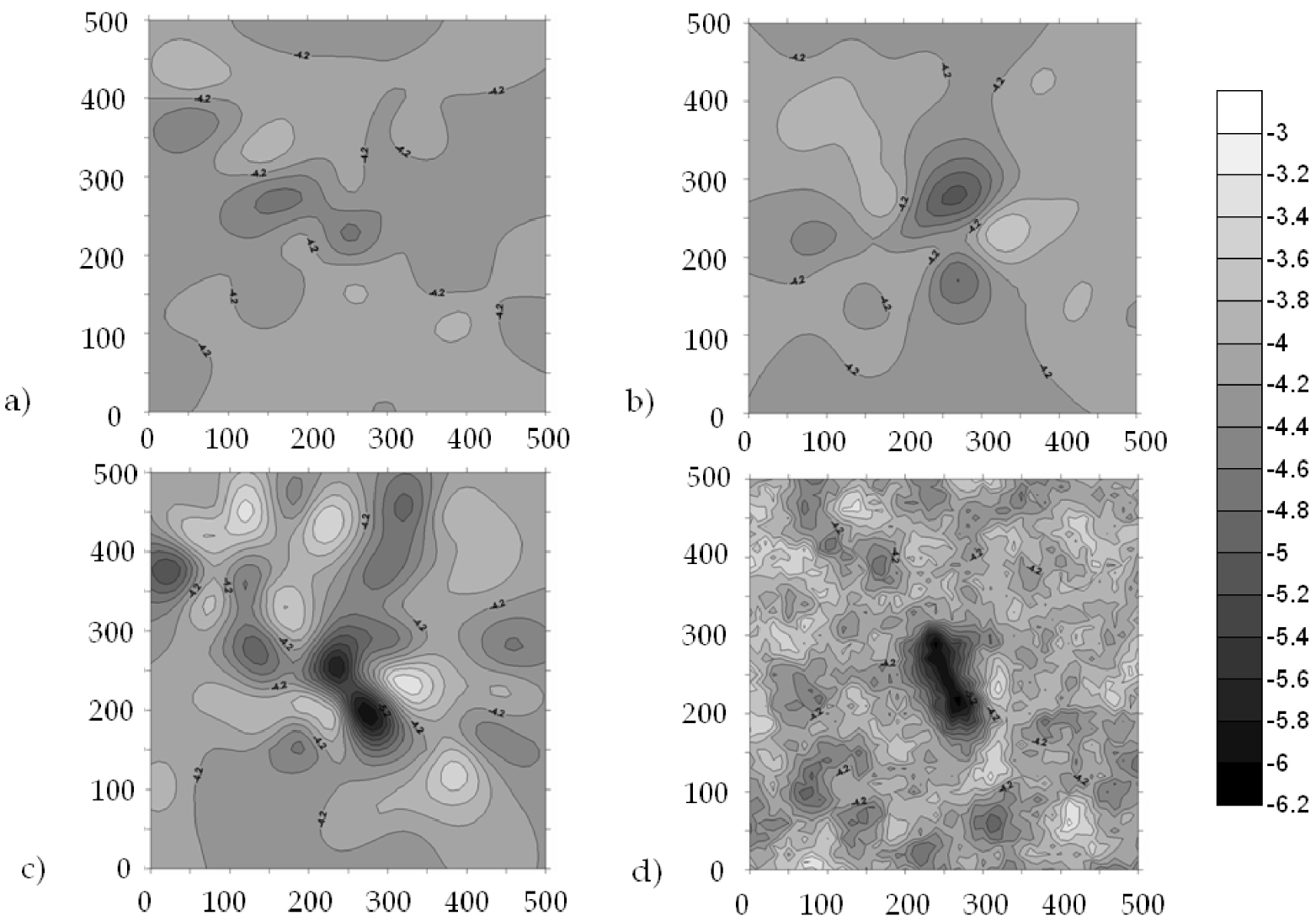
The results remain similar on the study zone (Table 2c): with head data from the N–S flow, the MAE and the RMSE increase compared with kriging and they decrease sharply with head data from the W–E flow only. Once again, MAE and RMSE are minimal by crossing W–E and NW–SE flows. For all configurations, the RMSSE is lower than for the homologous case for the extended area.
However on these three heterogeneous areas, the available data do not allow estimating the transmissivity accurately.
3.4. Interpreting the results
The improvement of the precision of the transmissivity with head data from two flows can be explained by returning to the stream lines. It is known [Emsellem and de Marsily 1971; de Marsily et al. 2000] that the solution of the inverse problem for the steady-state flow equation, including a recharge or pumping, is written
The transmissivity at any point of this stream-tube can thus be deduced from the transmissivity at s0. Formally, knowing the transmissivity along a line intersecting all the stream-tubes allows deducing the transmissivity everywhere in the field. In the case of two flows with nonparallel stream lines, knowing the transmissivity in a single point allows deducing the transmissivity everywhere in the field; see for example Castelier [1995].
In practice, the head is not known exhaustively but estimated, and the same for the stream-tubes. The estimate of transmissivity is therefore uncertain.
3.5. Practical conclusions from these synthetic cases
This synthetic example leads to practical conclusions on estimating transmissivity field:
- sufficiently close head measurements allow estimating the head gradient, which is more useful for the accuracy than isolated head values;
- “crossing” two steady-state flows improves the accuracy of transmissivity estimation;
- this flow crossing is useful for detecting heterogeneities of a transmissivity field. However, transmissivity data have to be numerous enough for precisely delineating the heterogeneities;
- since the accuracy of the estimation depends on the main flow direction, the same applies to the “optimal” implantation of the data.
4. Conclusive remarks
4.1. Towards more complex flow conditions
In many cases, the hypothesis of a macroscopically linear two-dimensional flow is unsuitable.
Roth et al. [1998] developed a flexible and general approach in order to avoid excessive simplifications. The principle is to come back to conventional hydrogeological modelling, using a flow simulator. A set of geostatistical (non-conditional) simulated transmissivity fields is used as input of a flow simulator. The set of associated output results (head, concentration) is used to calculate the explicitly nonstationary covariance C(x,x′) or variogram 𝛾(x,x′) of the variable of interest. These nonstationary “numerical” simple and cross covariances or variograms of transmissivity and head are used to estimate by cokriging the transmissivity from transmissivity and head data. However an anamorphosis or at least a logarithmic transformation allows avoiding negative transmissivity estimates. Pannecoucke [2020] generalised this “numerical variogram” to transient flow, for mapping radionuclide activity.
To account for the non-linearity between concentration and hydraulic conductivity field, Schwede and Cirpka [2010] show that a Monte-Carlo approach is preferable for conditioning hydraulic conductivity fields by steady-state concentration measurements.
4.2. Back transformation of estimated log-transmissivity
According to de Marsily et al. [2005] “One also needs to apply Kriging with some rigor on the log-transformed transmissivity values, in order to estimate geometric mean values and not arithmetic means. Back-transforming the kriged lnT into T values must also be done correctly, i.e. simply as T = exp(lnT) without any additional factor using the variance of the estimation error to supposedly correct an assumed estimation of the median rather than of the mean, as is sometimes erroneously done”.
Another question is that of the support of the estimate: is kriging “punctual”, that is to say that the transmissivity has to be estimated on the same support as the transmissivity data, or is a larger support chosen, in which case an equivalent transmissivity is sought? However, except in the very special case of a stratified medium with a flow parallel to the stratification, the permeability is not additive. The equivalent block-permeability lies within the harmonic and the arithmetic mean of sub-block permeabilities [Matheron 1993; Delhomme and de Marsily 2005]. In the special case of lognormal transmissivity with isotropic variogram, and with some additional hypotheses, Matheron [1967] has shown that the equivalent transmissivity is the geometric mean. Coming back to the estimated transmissivity simply consists thus to exponentiate the estimated log-transmissivity.
In practice, the regularisation similarly has to be carried out on the log-transmissivities, and the result is simply exponentied. The bounds of the uncertainty interval can be calculated in the same way from the bounds of this interval on logarithmic estimates.
In a more thorough approach, tensor transmissivity fields should be estimated.
4.3. Biased flow predictions computed on estimated transmissivity fields
However it is known that the (co)kriging “smoothes” map of the estimated values, whose spatial variability therefore differs from that of the real values. The non-linear calculations performed on an estimated transmissivity field (by (co)kriging or any other estimator, linear or not) is biased. A simulation based approach is then required.
The cokriging of log-transmissivity by log-transmissivity and head measurements however allows the direct conditioning of log-transmissivity simulations to these data. When the validity of the linearisation of the flow equation is not verified, especially when the head gradient cannot be assumed to be constant at the macroscopic scale, the simple and crossed “numerical variogram” between log-transmissivity and head (perturbations) provides a consistent bivariate model, which is compatible with the boundary conditions where these are known [Schwede and Cirpka 2010; Pannecoucke et al. 2020]. However, the results shown here in the simplified case of the linearized flow equation remain useful in the general case: “crossing” two quasi steady-state flows (two seasonal situations for example) should improve characterising transmissivity heterogeneities.
Declaration of interests
The authors do not work for, advise, own shares in, or receive funds from any organization that could benefit from this article, and have declared no affiliations other than their research organizations.
Acknowledgments
The authors warmly thank Jean-Pierre Delhomme for initiating and contributing to the study of flow crossing. They also thank Marco De Lucia for his initial contribution to review the theoretical part of this study and the reviewers for their comments that helped to better highlight the results.