

 CC-BY 4.0
1. Introduction: climate modelling and its possible future
Earth system science has become an area of great growth caused by contemporary concerns about climate change. Taking the global average surface temperature as a measure of the climate state, we can ask the following question, to what degree are we living in a particular era in the geological history of the planet, and whether its recent variations have a precedent in the geological history of our planet. To do this, let's start by looking at temperature changes over the past 500 million years, Figure 1.
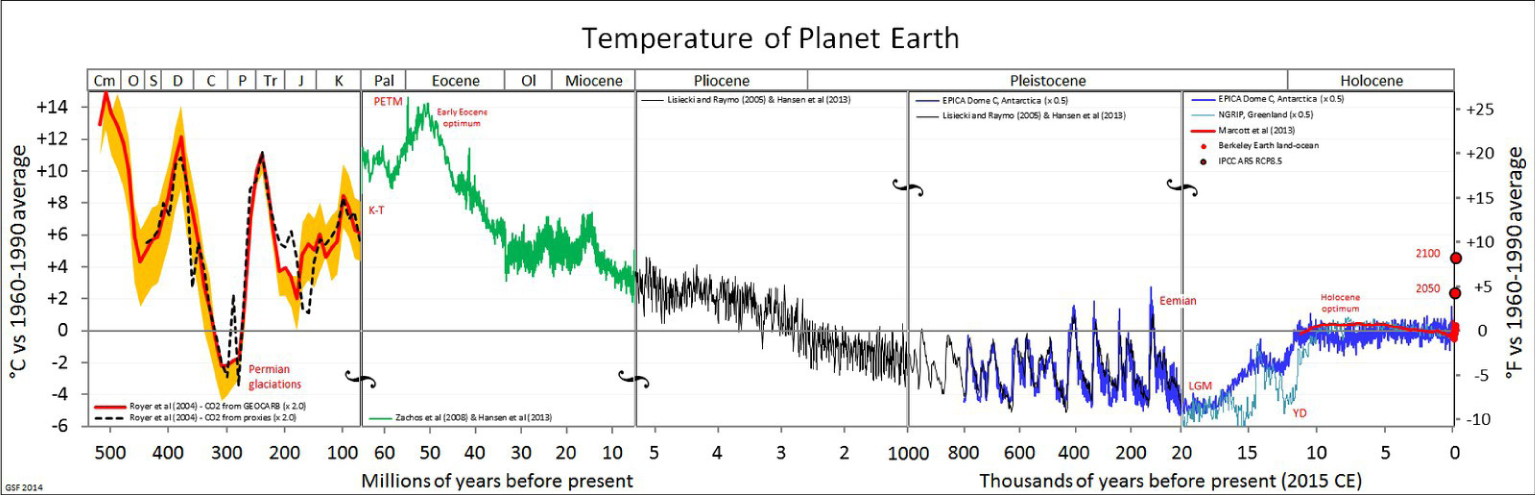
History of global temperature. Source: Wikipedia
This reconstruction of the global temperature is based on the interpretation of many proxies that are beyond the scope of this article (e.g. see the discussion of this figure in the famous blog RealClimate,1).
The major events presented here are undisputed: for example, the Paleocene-Eocene Thermal Maximum (PETM) of about 50 million years ago; the large temperature oscillations leading to ice ages, which began about 1 million years ago, and the recent period of relative stability beginning about 10,000 years ago. We see, of course, the significant rise in temperatures at the very end of the register, representing the period of very strong human influence on the planet, starting with the industrial revolution. This increase in temperature may take us out of the temperature comfort zone that humanity has experienced since its sedentarisation [Xu et al. 2020], which represents the entire history of sedentary human life: the scenery, with agriculture, cities, and civilisation. H. Sapiens predates this human "niche", of course, but before this period he was nomadic, following the edge of the ice which periodically covered the land masses. Many events in the history of human migration coincide with major climatic change, e.g. the meeting between Neanderthals and modern humans [Timmermann 2020]. It is also not the first time that we have seen historical events that have an effect on the global climate: the arrival of Europeans in the New World has led to a "great death" of indigenous people that has also left its mark on the carbon balance and temperature [Koch et al. 2019].
Let us now focus on the recent increase in temperature (Figure 1). The major debates around climate change policy today revolve around the causes and consequences of this temperature change, and what it means for life on the planet. It is perhaps underestimated the extent to which these results depend on simulations of the entire planet: the dynamics of the atmosphere and ocean, and their interactions with the marine and terrestrial biosphere. Here we show, for example, the SPM.7 figure.of the latest report of the Intergovernmental Panel on Climate Change (IPCC), published in 2013 (Stocker et al. 2013] (the next report, AR6, is currently being drafted). In this figure, reproduced here (Figure 2), we see the ability of models to reproduce the climate of the 20th century. For the 21st century, two "scenarios" are presented: one, named RCP8.5, representing a world without much effort to curb CO2 emissions, the other, RCP2.6, showing the thermal pathway of a world subject to climate change mitigation policies.
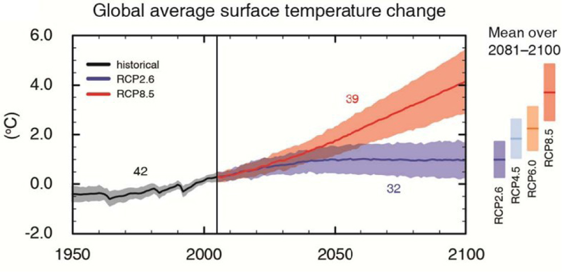
Figure SPM.7 of IPCC AR5 [Stocker et al. 2013].
It may not be obvious enough how much these numbers are due to models and simulations. As we shall see, we have spent many decades constructing models, which are mainly based on well-known physical laws, of which many aspects are nevertheless still imperfectly mastered. The coloured bands around the curves represent imperfect knowledge or "epistemic uncertainty". We estimate the limits of this uncertainty by asking different scientific groups to construct different independent models (the number next to the curves in Figure 2 represents the number of models participating in this exercise). The underlying dynamics are " chaotic ", which represents another form of uncertainty.
The role of different types of uncertainty, both internal and external, has often been analysed (see the example in Figure 4 of [Hawkins and Sutton 2009], often cited). It is studied by running simulations that sample all forms of uncertainty. Such sets of simulations are also used for studies on the detection of climate change in a system with natural stochastic variability and its attribution to natural or human influence, for example to ask whether a certain event such as a heatwave (e.g. [Kew et al. 2019]), can be attributed to climate change. For such studies, we depend on models to provide us with "counterfactuals " (possible states of the system that have never occurred), where we simulate fictitious Earth planets without human influence on the climate, which cannot be observed.
The central role of numerical simulation in understanding the Earth system dates back to the dawn of modern computing, as described below. These models are based on a solid foundation of physical theory; therefore, we keep faith in them when simulating counterfactuals that cannot be verified by observations. In parallel, many projects aim to build learning machines, the field of artificial intelligence. These two major trends in modern computing began with key debates between pioneers such as John von Neumann and Norbert Wiener. We will show how these debates took place at a time when numerical simulation of weather and climate was developing. These are being revisited today, while we have the same debates today, confronting data science with physical science, the detection of shapes and patterns ("pattern recognition ") in data versus the discovery of underlying physical laws. Below we will show how new data technologies can lead to a new synthesis of data physics and science.
2. A brief history of meteorology
The history of numerical weather and climate prediction is almost exactly coincident with the history of digital computing itself [Balaji 2013]. This story has been vividly told by historians [Dahan-Dalmedico 2001; Edwards 2010; Nebeker 1995], as well as by the participants themselves [Platzman 1979; Smagorinsky 1983], who worked alongside John von Neumann since the late 1940s. The development of dynamic meteorology as a science in the 20th century has been told by practitioners (e.g. [Held 2019; Lorenz 1967]), and we would not dare to try to do it better here. We will come back to this story below, because some of the first debates are resumed today and are the subject of this investigation. Over the past seven decades, numerical methods have become the heart of meteorology and oceanography. For weather prediction a "quiet revolution" [Bauer et al. 2015] has given us decades of steady advances based on numerical models that integrate the equations of motion to predict the future evolution of the atmosphere, taking into account thermodynamic and radiative effects and time-evolving boundary conditions, such as the ocean and the land surface.
The pioneering studies of Vilhelm Bjerknes (e.g. [Bjerknes 1921]) are often used as a marker to signal the beginning of dynamic meteorology, and we choose to use Vilhelm Bjerknes to highlight a fundamental dialectic that has animated the debate from the beginning, and to this day, as we shall see below. Bjerknes pioneered the use of partial differential equations (the first use of the "primitive equations") to represent the state of circulation and its time evolution, but closed-form solutions were hard to come by. Numerical methods were also immature, especially with regard to the study of their stability as seen in Richardson's [1922] failed attempts involving thousands of people doing calculations on paper. Finally abandoning the equations-based approach (global data becoming unavailable during war and its aftermath also played a role), Bjerknes reverted to making maps of air masses and their boundaries [Bjerknes 1921]. Forecasting was often based on a vast library of paper maps to find a map that resembled the present, and looking for the following sequence, what we would today recognise as Lorenz’s[1969] analogue method. Nebeker has commented on the irony that Bjerknes, who laid the foundations of theoretical meteorology, was also the one who developed practical forecasting tools "that were neither algorithmic nor based on the laws of physics" [Nebeker 1995].
We see here, in the sole person of Bjerknes, several voices in a conversation that continues to this day. One conceives of meteorology as a science, where everything can be derived from the first principles of classical fluid mechanics. A second approach is oriented specifically toward the goal of predicting the future evolution of the system (weather forecasts) and success is measured by forecast skill, by any necessary means. This could, for instance be by creating approximate analogues to the current state of the circulation and relying on similar past trajectories to make an educated guess of future weather. One can have an understanding of the system without the ability to predict; one can have skillful predictions innocent of any understanding. One can have a library of training data, and learn the trajectory of the system from it, at least in some approximation or probabilistic sense. If no analog exists in the training data, no prediction is possible. What was later called "subjective" forecasts depended a lot on the experience and recall of the meteorologist, who was generally not well versed in theoretical meteorology, as Phillips remarks (1990). Rapidly evolving events without obvious precursors in the data were often missed.
Charney's introduction of a numerical solution to the barotropic vorticity equation, and its execution on ENIAC, the first operational digital computer [Charney et al. 1950], essentially led to a complete reversal of fortune in the race between physics and pattern recognition. Programmable computers (where instructions were loaded in as well as data) came soon after, and the next landmark calculation of Phillips [1956] came soon thereafter.
It was not long before forecasts based on simplified numerical models outperformed subjective forecasts. Forecasting skill, measured (as today!) by errors in the 500 hPa geopotential height, was clearly better in the numerical predictions after Phillips' breakthrough (see Figure 1 in [Shuman 1989]). It is now considered a well-established fact that forecasts are based on physics: Edwards [2010] remarks that he found it hard to convince some of the scientists he met in the 1990s that it was decades since the founding of theoretical meteorology before simple heuristic and theory-free pattern recognition became obsolete in forecast skill.
Using the same methods run for very long periods of time (what von Neumann called "infinite forecast " [Smagorinsky 1983]), the field of climate simulation developed over the same decades. While simple radiative arguments for CO2-induced warming were advanced in the 19th century, numerical simulation led to the detailed understanding which includes the dynamical response of the general circulation to an increase in atmospheric CO2 (e.g. [Manabe and Wetherald 1975]). Models of the ocean circulation had begun to appear (e.g. [Munk 1950]) showing low-frequency variations showing low-frequency (by atmospheric weather standards) variations, and the significance of atmosphere-ocean coupling [Namias 1959]. The first coupled model of Manabe and Bryan [1969] came soon thereafter. Numerical meteorology also serendipitously led to one of the most profound discoveries of the latter half of the 20th century, namely that even completely deterministic systems have limits to the predictability of the future evolution of the system, the famous "strange attractor", a mark of "chaos" [Lorenz 1963]. Simply knowing the underlying physics does not translate to an ability to predict beyond a point. Long before Lorenz, Norbert Wiener had declared that it would be a "bad technique" [Wiener 1956] to apply smooth differential equations to a nonlinear world where errors are wide and the precision of observations is small. Lorenz demonstrated this in a deterministic but unpredictable system of only three variables, in one of the most beautiful and profound recent results of physics.
However, the statistics of weather fluctuations in the asymptotic limit could still be usefully studied [Smagorinsky 1983]. Within a decade, such models were the basic tools of the trade for studying the asymptotic equilibrium response of Earth system to changes in external forcing, became the new field of computational climate science.
The practical outcomes of these studies are the response of the climate to anthropogenic phenomena. CO2 raised public alarm with the publication of the Charney Report in 1979 [Charney et al. 1979]. Computational climate science, now with planetary-scale societal ramifications, became a rapidly growing field expanding across many countries and laboratories, which could all now aspire to the scale of computing required to work out the implications of anthropogenic climate change. There was never enough computing: it was clear, for example, that the representation of clouds was a major unknown in the system (as noted in the Charney Report) and was (and still is, see [Schneider et al. 2017]) well below the spatial resolution of models able to exploit the most powerful computers available. The models were resource-hungry, ready to soak up whatever was provided to them for the calculation. A more sophisticated understanding of the Earth system also began to bring more processes into the simulations, now an integrated whole with physics, chemistry and biology components. The calculation cost (not to mention energy and carbon footprint) of these simulations becomes significant [Balaji et al. 2017]. Yet, recalcitrant errors remain. The so-called "double ITCZ" bias for example has remained stubbornly resistant to any amount of reformulation or tuning across many generations of climate models [Li and Xie 2014; Lin 2007; Tian and Dong 2020]. It is contended by many that no amount of fiddling with parameterizations can correct some of these “recalcitrant ” biases, and that only direct simulation is likely to lead to progress (e.g. [Palmer and Stevens 2019], Box 2).
The revolution begun by von Neumann and Charney at the IAS, and the subsequent decades of exponential growth in computing have led to tremendous leaps forward as well as more ambiguous indicators of progress. What initially looked like a clear triumph of physics allied with computing and algorithmic advances now shows signs of stalling, as the accumulation of "details" in the models — both in resolution and complexity — leads to some difficulty in the interpretation and mastery of model behaviour. This is leading to a turn in computational climate science that may be no less far-reaching than the one wrought in Princeton in 1950.
Just around the time the state of play in climate computing was reviewed [Balaji 2015], the contours of the revival of artificial neural networks (ANNs) and machine learning (ML) were beginning to take shape. As noted in Section 2, ANNS existed alongside the von Neumann and Charney models for decades, but may have languished as the computing power and parallelism were not available. The new processors emerging today are ideally suited to ML: the typical deep learning (DL) computation consists of dense linear algebra, scalable almost at will, able to reduce the memory bandwidth at reduced precision without loss of performance. Processors such as TPU (the tensor processing unit) showed themselves capable of running a typical DL workload at close to the maximum performance of the chip [Jouppi et al. 2017].
While the promises of neural networks failed to materialise after their discovery in the 1960s (e.g., the "perceptron" model of [Block et al. 1962]), these methods have undergone a remarkable resurgence in many scientific fields in recent years, while conventional approaches stalled. While the meteorological community may have initially been somewhat reticent (for reasons outlined in [Hsieh and Tang 1998]), the last 2 or 3 have witnessed a great efflorescence of literature applying machine learning or ML — as it is now called — in Earth system science. We argue in this article that this represents a sea change in computational Earth system science that rivals the von Neumann revolution. Indeed, some of the current debates around machine learning — pitting "model-free" methods against '"interpretable AI"2 for example — recapitulate those that took place in the 1940s and 1950s.
3. Learning physics from data
Recall V. Bjerknes’s turn away from theoretical meteorology upon finding that the tools at his disposal were not adequate to the task of making predictions from theory. It is possible that the computational predicament we now find ourselves in is a historical parallel, and we too shall turn toward practical, theory-free predictions. An example would be the prediction of precipitation from a sequence of radar images [Agrawal et al. 2019] (essentially, extrapolating various optical transformations such as translation, rotation, stretching, intensification) is compared and found competitive with persistence and short term model-based forecasts. ML methods have shown exceptional forecast skill at longer timescales, including breaking through the "spring barrier" (this is the name given to a reduction in forecast skill in models initialised prior to boreal spring) in the ENSO phenomenon predictability [ham et al. 2019]. Interestingly, the Lorenz analogue method [1969] also shows longer term ENSO skill (with no spring barrier) compared to dynamical models [Ding et al. 2019], a throwback to the early days of forecasting as described in Section 2. These and other successes in the purely "data-driven" field (though the ENSO papers cited here use model outputs as training data); forecasting have led to speculation in the media that ML might indeed make physics-based forecasting obsolete (see for example, "Could Machine Learning Replace the Entire Weather Forecast System?3 in HPCWire). ML methods (in this case, recurrent neural networks) have also shown themselves capable of reproducing a time series from canonical chaotic systems with predictability beyond what dynamical systems theory would suggest [Pathak et al. 2018] which indeed makes a claim to be “model-free”, or [Chattopadhyay et al. 2020]). Does this mean we have come full circle on the von Neumann revolution, and return to forecasting from pattern recognition rather than physics? The answer of course is contingent on the presumption that the training data in fact is comprehensive and samples all possible states of the system. For the Earth system, this is a dubious proposition, as there is variability on all time scales, including those longer than the observational record itself, the satellite era for instance. A key issue for all data-driven approaches is that of generalisability beyond the confines of the training data.
Turning to climate, we look at the aspects of Earth system models that while broadly based on theory, are structured around an empirical formulation of principles. These are areas obviously ripe for a more data-driven approach. These models are often based on the parameterised components of the model that deal with "sub-gridscale" physics below the truncation imposed by the discretisation. A key feature of geophysical fluid flow is the 3-dimensional turbulence cascade continuous from planetary scale down to the Kolmogorov length scale (see for example [see e.g., Nastrom and Gage 1985], Figure 1), which must be truncated somewhere for a numerical representation. ML-based representation of subgrid turbulence is one area receiving considerable attention now [Duraisamy et al. 2019]. Other sub-gridscale aspects particular to Earth system modeling exist, where ML could play a role, including radiative transfer and the representation of clouds
ANNs have the immediate advantage of often being considerably faster than the component they replace [Krasnopolsky et al. 2005; Rasp et al. 2018]. Further, the calibration procedures of [Hourdin et al. 2017] are very inefficient with full models, and may be considerably accelerated using emulators derived by learning [Williamson et al. 2013].
ML nonetheless poses a number of challenging questions that we are now actively addressing. The usual problems of whether the data is representative and comprehensive, and on generalisability of the learning, continue to apply. There is a conundrum in deciding where the boundary between being physical knowledge driven and data driven lies. We outline some key questions being addressed in the current literature. We take as a starting point, a particular model component (such as atmospheric convection or ocean turbulence) that is now being augmented by learning. Do we take the structure of the underlying system as it is now, and use learning as a method of reducing parametric uncertainty? Emerging methods potentially do allow us to treat structural and parametric error on a common footing (e.g. [Williamson et al. 2015]), but we still may choose to go either structure-free, or attempt to discover the structure itself. [Zanna and Bolton 2020].
If we divest ourselves of the underlying structure of equations, we have a number of issues to address. As the learning is only as good as the training data, we may find that the resulting ANN violates some basic physics (such as conservation laws), or does not generalise well [Bolton and Zanna 2019]. This can be addressed by a suitable choice of basis in which to do the learning, see Zanna and Bolton [2020]. A similar consideration was seen in [O'Gorman and Dwyer 2018], which when trained on current climate failed to generalie to a warmer climate, but the loss of generalisability could be addressed by a suitable choice of input basis. Ideally, we would like to go much further and actually learn the underlying physics.
There have been attempts to learn the underlying equations for well-known systems [Brunton et al. 2016; Schmidt and Lipson 2009] and efforts underway in climate modeling as well, to learn the underlying structure of parameterisations from data. Finally, we pose the problem of coupling. We have noted earlier the problem of calibration of models, which is done first at the component level, to bring each individual process within observational constraints, and then in a second stage of calibration against systemwide constraints, such as top of atmosphere radiative balance [Hourdin et al. 2017]. The issue of the stability of ANNs when integrated into a coupled system is also under active study at the moment (e.g. [Brenowitz et al. 2020]). The first step is to choose the unit of learning: should it be an individual process, or the whole system?
4. Summary
We have highlighted in this article a historical progression in Earth system modeling, in which the von Neumann revolution allowed us to move from pattern recognition to direct numerical manipulation of the equations of physics.
We have described how statistical machine learning of massive amounts of data offers the possibility of drawing directly on observations to predict the Earth system, a transition that is potentially as far-reaching as that of von Neumann.
At first glance, it may appear as though we are turning our backs on the von Neumann revolution, going back from physics to simply seeking and following patterns in data. While such black-box approaches may indeed be used for certain activities, we are seeing many attempts to go beyond those, and ensure that the learning algorithms do indeed respect physical constraints even if not present in the data. Science is of course observations based on observations. But "theory is loaded with data, and data is loaded with theory", according to the words pronounced by the philosopher Pierre Duhem. Edwards [2010] proposed that the same idea applies to models: models are loaded with data, but data is also loaded with models. We see this clearly with respect to climate data, which is often based on so-called 'reanalysis', a global dataset, created from sparse observations and extrapolated using theoretical considerations. An interesting recent result [Chemke and Polvani 2019] shows this conundrum, in which it turns out that the models of the future are correct but that the data of the past (i.e. the reanalyses) are wrong!
The field also needs models to build "counterfactuals" against which current reality is compared. This means that even learning algorithms must use model-generated results as training data, rather than observations. The results of machine learning from this simulated data will learn to emulate them, thus moving from simulation to emulation.
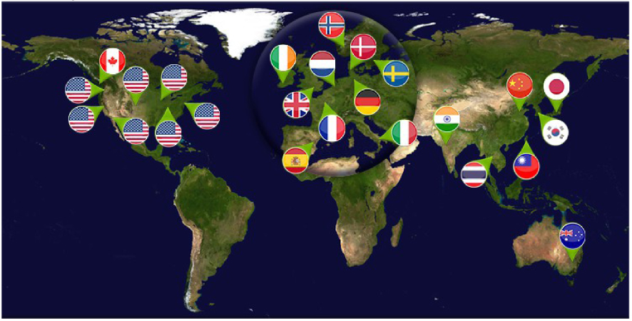
The global Earth System Grid Federation network.
This has already become evident in recent trends, in which we see simulated data becoming comparable in size to the massive amounts of satellite observation data [Overpeck et al. 2011]. We see in Figure 3 the new "vast machine" of data across the world from distributed simulations for the IPCC, for the current assessment following that of Figure 2. It is imperative that this data is properly labelled and stored and therefore likely to be studied by machine learning tools. This global data infrastructure shows the possibilities of a new synthesis of physical knowledge and big data: through the emulation of simulated data, we will try to extract physical knowledge about the state of the planet and the ability to predict its future evolution.
Funding
V. Balaji is supported by the Cooperative Institute for Modeling the Earth System, Princeton University, under Award NA18OAR4320123 from the National Oceanic and Atmospheric Administration, U.S. Department of Commerce, and by the Make Our Planet Great Again French state aid managed by the Agence Nationale de Recherche under the “Investissements d’avenir” program with the reference ANR-17-MPGA-0009.
The statements, findings, conclusions, and recommendations are those of the authors and do not necessarily reflect the views of Princeton University, the National Oceanic and Atmospheric Administration, the U.S. Department of Commerce, or the French Agence Nationale de Recherche. The author(s) declare that they have no competing interests.
Acknowledgments
I thank Ghislain de Marsily, Fabien Paulot, and Raphael Dussin for their careful reading of the inital versions of this article, which considerably improved the manuscript. I thank the French Académie des sciences and the organisers of the colloquium "Facing climate change, the field of possibilities" in January 2020, for giving me the opportunity to participate and contribute to this special issue.
1http://www.realclimate.org/index.php/archives/2014/03/can-we-make-better-graphs-of-global-temperature-history, retrieved on July 31, 2020.
2AI, or artificial intelligence, is a term we shall generally avoid here in favour of terms like machine learning, which emphasise the statistical aspect, without implying insight.
3https://www.hpcwire.com/2020/04/27/could-machine-learning-replace-the-entire-weather-fore retrieved on July 31, 2020.