


 CC-BY 4.0
1. Introduction
Gansu Province, located in inland China, lies at the intersection of the Qinghai-Tibet Plateau, the Loess Plateau, and the Inner Mongolia Plateau. This region is characterized by its complex geological structures, diverse landforms, and fragile ecological environment. Frequent earthquakes and concentrated rainfall make it highly susceptible to geological hazards such as collapses, landslides, and debris flows (Meng and Derbyshire, 1998; F. Zhang and X. Huang, 2018; Fan, Scaringi, et al., 2019; D. Peng et al., 2019; Y. Xu et al., 2020). Among its cities, Tianshui is the second largest in Gansu Province and lies on the southern edge of the Loess Plateau. The area’s bedrock primarily consists of mudstone, overlain by loess, forming a geologically unstable setting highly sensitive to rainfall (Z. L. Zhang et al., 2020; T. Qi et al., 2021). Human activities such as irrigation and land reclamation significantly influence soil–water interactions, further destabilizing slopes (F. Zhang and G. Wang, 2018; Jia et al., 2023; Lan et al., 2023). The Fengjiaping Landslide, located in the Tianshui region, is a representative loess–mudstone interface landslide triggered by multiple factors. Assessing its risk requires a comprehensive understanding of the hydromechanical processes that drive its activity.
Moisture-induced landslides are often triggered by water infiltration in the unsaturated zone, groundwater table fluctuations, preferential flow paths, and their complex interactions (Sorbino and Nicotera, 2013; Fan, Q. Xu, et al., 2017; Whiteley et al., 2019; Y. Xu et al., 2020). During rainfall or artificial irrigation events, infiltrating water rapidly increases pore water pressure and soil moisture, weakening the shear strength and raising the likelihood of slope failure. Notably, shallow landslides may initiate before full soil saturation is reached (Sorbino and Nicotera, 2013; P. Li et al., 2016; Z. Yang et al., 2017; Filho and Fernandes, 2019; Hu, Mo, et al., 2021). Conversely, landslides may also occur under fully saturated conditions due to aquifer variations caused by water recharge, even in the absence of rainfall (Tu et al., 2010). The critical roles of groundwater flow and soil moisture in these processes underscore the importance of monitoring their spatial and temporal variations to identify high-risk zones and support risk management.
Understanding landslides requires an integrated approach that considers the complex interactions within the critical zone, particularly in regions like Tianshui. Monitoring rainwater infiltration and hydrodynamic processes often involves hydrological and deformation measurements. Conventional techniques include measuring pore water pressure, matric suction, soil moisture, and groundwater levels, as well as stress–strain and surface deformation monitoring (e.g., Lourenço et al., 2006; Schulz et al., 2009; Terajima et al., 2014; Jiang et al., 2017; Lu et al., 2024). However, these approaches are largely point-based or surface measurements, offering limited resolution of the internal dynamics of landslides. Given the heterogeneous nature of water flow within sliding masses, no single traditional technique can fully capture their spatial and temporal complexity.
Geophysical methods provide valuable tools for imaging subsurface structures and delivering higher spatial information than point-based measurements. Among these, Direct-Current Electrical Resistivity Tomography (DC ERT) is widely applied in landslide studies due to its sensitivity to water content. The availability of open-source and user-friendly inversion software such as Res2DInv (Loke and Barker, 1996; Loke, 2020), BERT (Rücker, Günther and Spitzer, 2006; Günther et al., 2006), pyGIMLi (Rücker, Günther and Wagner, 2017), and ResIPy (Blanchy et al., 2020), has further promoted its use in landslide research (e.g., Caris and Van Asch, 1991; Lapenna, Lorenzo, Perrone, Piscitelli, Sdao, et al., 2003; Lapenna, Lorenzo, Perrone, Piscitelli, Rizzo, et al., 2005; Colangelo et al., 2006; Perrone et al., 2014; Uhlemann et al., 2017; D. Peng et al., 2019). For instance, Gance et al. (2015) applied the open-source BERT framework to correct fissure effects in resistivity pseudosections, improving interpretation reliability. More recently, Jabrane et al. (2023) combined ERT with vertical electrical soundings using pyGIMLi and BERT to delineate sliding surfaces, underscoring ERT’s potential for landslide monitoring and hazard assessment. Low resistivity is often associated with highly saturated soils and therefore related to slope instability (Szalai et al., 2017; Zhao et al., 2020; X. Wang et al., 2022; F. Zhang, G. Wang and J. Peng, 2022). In the Loess Plateau, however, resistivity is also influenced by high salinity, clay content, and structural features such as fissures and loess caves (Waxman and Smits, 1968; Jougnot, Ghorbani, et al., 2010; Revil, Coperey, et al., 2017; T. Zhang et al., 2019; Mendieta et al., 2021; Y. Qi and Wu, 2022). These complexities highlight the need to combine geophysical methods with localized geological knowledge for reliable interpretation.
In addition to ERT, the self-potential (SP) method provides a passive approach for monitoring hydrogeological processes. SP measurements capture natural electric fields generated by infiltrating water, offering unique insights into subsurface water flow (Thony et al., 1997). Since the early 20th century, SP has been recognized for its potential in landslide monitoring, particularly due to its sensitivity to water saturation and water flow (Bogoslovsky and Ogilvy, 1977; Corwin, 1990). Recent studies show its promise as a supporting tool for early warning of rainfall-induced landslides, as it can detect water infiltration and preferential flow patterns (Haas and Revil, 2009; Yamazaki et al., 2017; Whiteley et al., 2019; Guo et al., 2022; Hu, Q. Huang, Tang, et al., 2024; Hu, Q. Huang, Han, Tao, et al., 2025; de Araújo et al., 2025). For example, in southern Italy, SP mapping has been successfully applied to investigate groundwater flow direction in landslide zones (Lapenna, Lorenzo, Perrone, Piscitelli, Sdao, et al., 2003; Colangelo et al., 2006). Additionally, Chambers et al. (2011), demonstrated the combined use of SP and ERT methods for investigating landslides in mudstone–sandstone formations.
Although this study shares methodological similarities with Chambers et al. (ibid.), it differs in several key aspects. First, the Fengjiaping Landslide represents a loess–mudstone contact surface landslide, dominated by Malan loess and fractured mudstone debris, where moisture infiltration and preferential flow were primary drivers of instability. This differs fundamentally from mudstone–sandstone settings as Chambers et al. (ibid.). Second, we applied an SP inversion approach based on the current continuity equation and incorporate ERT-derived conductivity models, in contrast to cross-correlation techniques used (e.g. Colangelo et al., 2006; Chambers et al., 2011; Hu, Q. Huang, Tang, et al., 2024). This approach ensures a more physically consistent interpretation of streaming current sources. Third, we integrated in-situ soil property measurements, including temperature, volumetric water content, and bulk electrical conductivity, which provided a stronger basis for interpreting geoelectrical anomalies.
In this study, we integrate passive SP and active ERT methods to investigate subsurface water flow paths and delineate possible water-rich zones that contribute to slope instability. By performing SP inversion combined with ERT results, we analyze SP source distributions and their implications for landslide processes. Using the Fengjiaping Landslide as a case study, our objective is to map subsurface water-storage areas and preferential pathways that may trigger reactivation. These geoelectrical approaches enhance the understanding of hydrological controls on landslides and provide a framework for improving risk assessment and mitigation strategies within the Earth’s critical zone.
2. Materials and methods
2.1. Study area
The Fengjiaping Landslide is an ancient landslide, shaped like a “circular chair”, measures approximately 840 m in length and an average width of 423 m, covering an area of 2.32 × 10⁵ m2 (Figure 1). It has an average thickness of 16 m, a total volume of 3.78 × 10⁶ m3, and a primary sliding direction of 245°. The elevation at the front edge of the landslide is 1390 m, while the rear edge rises to 1570 m, resulting in a relative elevation difference of 180 m. The overall slope of the landslide is 15.7°.
(a) Location of the investigation site; (b) the ancient Fengjiaping landslide marked by white line to indicate its boundary and its reactivation body with yellow shaded area (image from Google Earth); (c) the drill log (the red dot in b) conducted in April 22–23 of 2022. $Q_{4}^{\mathrm{ml}}$, $Q_{4}^{\mathrm{del}}$ and N denote artificially filled silt, Holocene deposits and the Neogene system, respectively.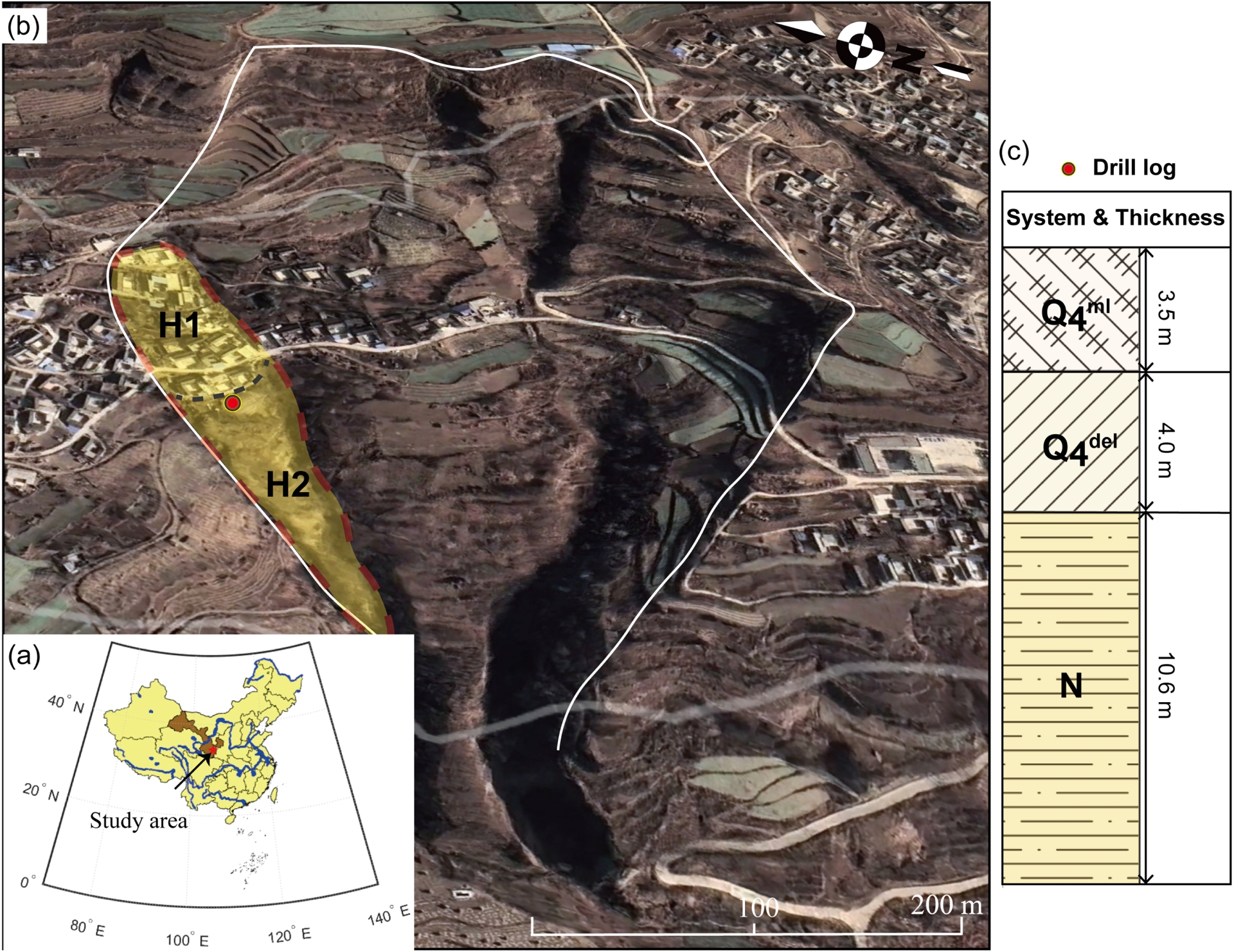
This ancient landslide has been reactivated due to the combined effects of rainfall, groundwater activity, and land use. The reactivated Fengjiaping Landslide is a medium-sized loess–mudstone contact surface landslide, displaying a “long tongue” shape planform and a stepped cross-sectional profile (Figure 1b). It features well-developed gullies along both sides of the landslide body (H1 and H2). The reactivated landslide has a front edge elevation of 1395 m and a rear edge elevation of 1532 m, with a relative height difference of 137 m. It spans 450 m in length, with an average width of 64.4 m, covering an area of 2.90 × 10⁴ m2. The reactivated landslide has an average thickness of approximately 8 m, a total volume of 2.32 × 10⁵ m3, a main sliding direction of 225°, and an average slope of 14.7°. The thicknesses of both the ancient and reactivated landslides were estimated based on borehole logging data. Since only two boreholes were available, located respectively within the H1 and H2 bodies, these thickness estimates are subject to uncertainty. Nevertheless, they provide first-order constraints on the internal structure of the landslide.
The study area is predominantly covered by Holocene strata of the Quaternary system. A borehole was drilled in the central region of the reactivated landslide body (34°24′36.641268′′N, 105°41′13.539480′′E) at an elevation of 1646.10 m above sea level on April 22–23, 2022 (Figure 1c). The drill logs indicate that the shallow zone primarily consists of artificially filled silt (Q$_{4}^{\mathrm{ml}}$), with increasing water content and heterogeneous soil texture at greater depths. The landslide accumulation mainly derives from Holocene deposits (Q$_{4}^{\mathrm{del}}$), predominantly composed of silty clay. Beneath these deposits, moderately weathered mudstone and sandy mudstone of the Neogene system (N) are exposed (Figure 1c). The integrity of the rock formation has been compromised by multiple vertical joints along the slope.
The deformation caused by the landslide has led to significant damage to residential properties (Figure 2). A visible gap between a house and its foundation underscores the ground displacement and movement caused by the landslide (Figure 2b). Within the landslide zone, one building shows extensive structural damage, with multiple fissures and large cracks along the walls, accompanied by a vertical displacement of approximately 1.70 m (Figure 2c). The exposed blue-gray mudstone layer in the gully of the slope is highly sensitive to water infiltration. Recharge into this layer reduces its mechanical strength, thereby accelerating slope destabilization. The interaction between infiltrating water and the mudstone layer plays a critical role in the reactivation and progression of the landslide. Understanding this relationship is essential for assessing the stability of the slope and predicting future risks.
The photos of (a) H2 body recorded by Da-Jiang Innovations (DJI) M300 drone, (b) and (c): house cracks, and (d) exposed mudstone layer in the gully of the landslide.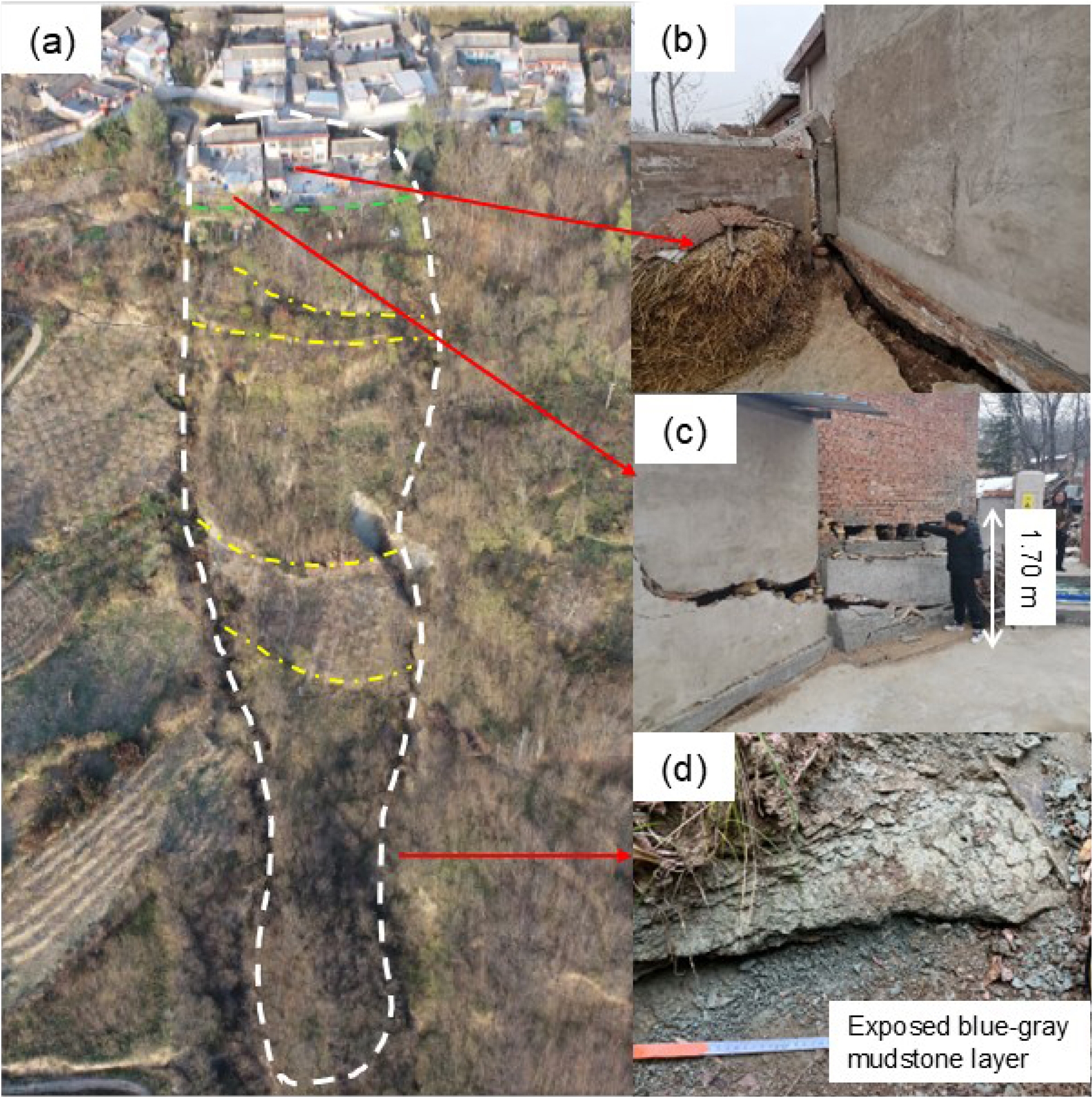
The primary trigger of the Fengjiaping landslide was attributed to rainfall. However, the presence of deep gullies and cracks complicates groundwater flow paths, leading to failures that are not always synchronized with rainfall events. Soils that are fully or partially saturated with water exhibit significantly lower electrical resistivity compared to their surroundings. Moreover, groundwater movement within the slope naturally generates SP signals. To identify the convergence zones of rainwater infiltration and detect hidden channels that facilitate dominant groundwater flow, we conducted geoelectrical measurements on the slope. By integrating ERT and SP methods, we inferred subsurface water flow paths, offering valuable insights into the hydrological processes that influence slope instability.
2.2. Data and methods
Drone-based LiDAR surveys were conducted across the Fengjiaping region to capture detailed topographic and surface feature data (Figure 3). The DJI M300 drone, equipped with Real-Time Kinematic (RTK) positioning and a DJI Zenmuse L1 LiDAR sensor, was used for data acquisition (Figure 3b). This LiDAR system can differentiate surface features such as soil, residential buildings, tree branches, and vegetation canopies by analyzing multiple echoes. The system provides an elevation accuracy of about 5 cm. The acquired LiDAR data were processed in DJI Terra software to generate a filtered point-cloud dataset, with buildings and vegetation removed. The processed data show topographic variability, with elevation differences in the study area exceeding 100 m (Figure 3a).
The observation system in the Fengjiaping landslide. (a) The digital elevation model (DEM) with measurement points using different techniques (Hu, Q. Huang, Han, Tao, et al., 2025); (b) Da-Jiang Innovations (DJI) M300 drone; (c) NI Compact DAQ for SP measurements; (d) ERT measurement.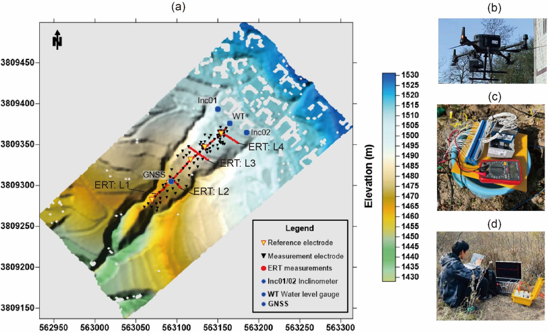
2.2.1. Monitoring data
Throughout 2023, we collected monitoring data, including atmospheric parameters from the Beidao station of National Oceanic and Atmospheric Administration (NOAA), water levels measured by a pressure-type water level gauge and elevation and azimuth angles recorded by inclinometers. The data show a correlation between temporal increases in precipitation and rising water table levels (Figure 4). Additionally, groundwater replenishment may also be influenced by the discharge from the Weihe River, a tributary of the Yellow River (J. Peng et al., 2015).
The monitoring data collected in the study area. (a) The hourly precipitation data collected from the Beidao station of NOAA; (b) the hourly displacement components measured by GNSS; (c) the depth of water table data; (d) the angle of azimuth and elevation data measured by two inclinometers; (e) the measured fracture width data by a crack meter located at lnc01.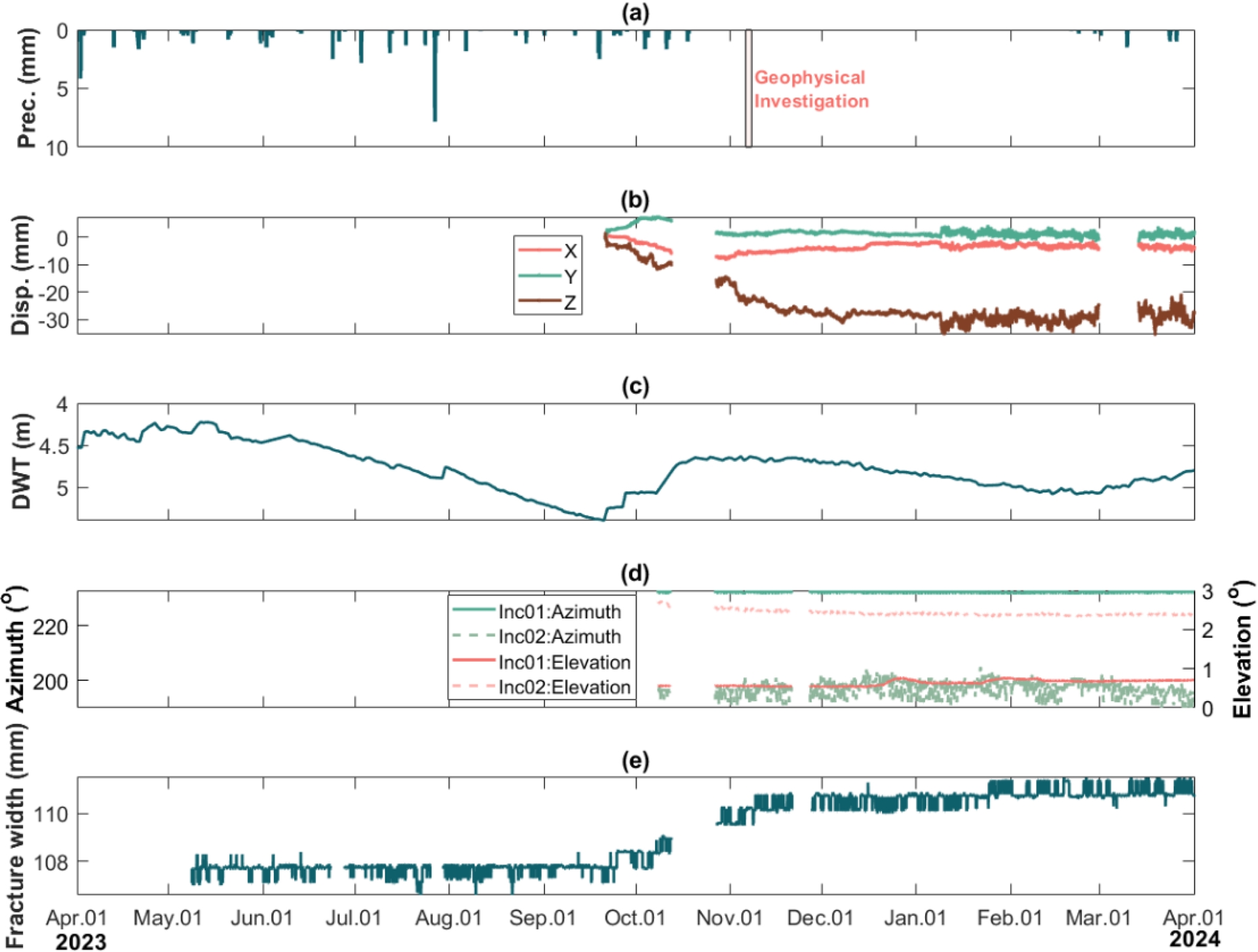
A Global Navigation Satellite System (GNSS) measuring station was installed in the southwestern part of the study area (Figure 3a). Two inclinometers (Inc01 and Inc02), located 47 m apart behind the residential buildings, recorded azimuth angles averaging 224.12° and 189.47°, respectively. The average elevation angles were 3.81° at Inc01 and 5.42° at Inc02. In October 2023, a notable rise in the water table (Figure 4c) coincided with an increase in fracture width near Inc01 (Figure 4e). By November, the northeastern edge of the slope exhibited general stability, while the central section of the study area experienced sliding (Figure 4b). This monitoring data highlights the spatiotemporal complexity of slope deformation, which appears to be strongly linked to the rising water levels.
2.2.2. Electrical resistivity tomography
To analyze the electrical structure of the Fengjiaping landslide, a primary ERT survey line (L1) was laid out downslope, with three additional survey lines (L2–L4) arranged perpendicularly to L1 (Figure 3a). The ERT instrument manufactured by Chongqing Jingfan Technology Co., Ltd. (China) was used in this experiment (Figure 3d). Before measurements, the grounding resistance of each electrode was checked to ensure all values were below 1 kΩ, minimizing data quality issues due to poor electrode contact. Table 1 provides details of the ERT profiles, including the number of electrodes, profile lengths, the number of data points, and the root mean square (RMS) misfit of inversion. Specifically, Line L1 employed a dipole–dipole array with a nominal electrode spacing of 2 m; however, due to the topographic variations in the steep-slope area, the actual electrode spacing was slightly larger. Lines L2–L4 used the Wenner array with an electrode spacing of 1 m.
Configuration of ERT surveys and inversion misfits
| Line no. | Number of electrodes | Length of survey line (m) | Number of datum points | Resulting misfit (RMS) |
|---|---|---|---|---|
| L1 | 60 | 118 | 570 | 1.95 |
| L2 | 20 | 19 | 57 | 1.53 |
| L3 | 30 | 29 | 135 | 1.22 |
| L4 | 30 | 29 | 135 | 1.93 |
For data processing, measurement points were corrected for elevation and distance, and the apparent resistivity values were calculated based on the actual electrode coordinates obtained using the RTK positioning. The ERT data were inverted using the open-source software ResIPy, which applies regularization inversion with linear filtering (Blanchy et al., 2020). In this framework, the inversion seeks a compromise between fitting the observed apparent resistivity data and minimizing spatial variations in the resistivity model. The choice of the initial reference model influences the convergence behavior and stability of the inversion. While ResIPy can automatically estimate an initial resistivity model from the apparent resistivity data, a uniform initial resistivity of 10 Ω⋅m was assigned to all survey lines to ensure a consistent starting point and facilitate comparison among profiles. Such a choice avoids introducing artificial contrasts related to differing initial models and promotes stable convergence (e.g., Tao, Han, X. H. Yang, et al., 2024).
The regularization parameter 𝜆 controls the trade-off between data misfit and model smoothness. Larger 𝜆 values favor smoother models at the expense of data fitting, whereas smaller values allow greater model variability but may lead to instability or overfitting (Loke, Dahlin, et al., 2014; Tao, Han, Ma, et al., 2024). In this study, 𝜆 was determined by the default adaptive optimization strategy in ResIPy, which automatically updates the regularization strength during the iterative inversion to balance data misfit reduction and model roughness. This approach provides a robust and objective means of selecting 𝜆 without manual tuning. The RMS errors of inversion on Lines L1, L2, L3, and L4 are 1.95, 1.53, 1.22, and 1.93, respectively. The raw ERT measurements on each survey line can be found in Hu, Q. Huang, Han, Tao, et al. (2025).
2.2.3. Self-potential
To investigate subsurface water flow within the deformation zone of the Fengjiaping landslide, a total of 86 sensors were strategically placed across the study area (Figure 3a). Given the extensive measurement area—spanning over 120 m—the site was divided into five smaller sub-regions. Each sub-region was equipped with one reference electrode and approximately 16 measurement electrodes (Figure S2 in the Supplementary Material). Continuous measurements were conducted in each sub-area at a sampling rate of 10 Hz for 20 min.
Data acquisition was facilitated using the National Instruments system (Figure 3c), where the input module connected sensors by differential connections to minimize common-mode interference. The control of SP measurements was achieved using an embedded LabVIEW program, which enabled the development of a multi-channel landslide monitoring system capable of synchronous observation and real-time data transmission. SP measurements utilized custom-built Pb-PbCl2 non-polarizable electrodes (Figure S4 in the Supplementary Material), which were pretested in the laboratory and showed excellent stability with minimal electrode potential differences (Hu, Q. Huang, Han, Y. Zhang, et al., 2025; S. Li et al., 2025).
Since SP signals are inherently weak and susceptible to environmental interference, several measures were implemented to ensure the accuracy and reliability of the data. First, the initial electrode range was measured in a saturated saline solution prior to each measurement, with electrodes submerged until readings stabilized. Second, to reduce surface noise, electrode pits were dug using a soil-lifting device, and electrodes were buried at a depth of 50 cm. After installation and wiring, electrical potential differences were checked with a multimeter to verify the accuracy of synchronous measurements before formal data collection. Finally, the electrical potential differences between reference electrodes in each sub-region were measured and used to calibrate all measurement points to a unified reference electrode. The raw monitoring and temperature- and electrode-corrected SP data are archived in Hu, Q. Huang, Han, Tao, et al. (2025). Further details of the SP pre-processing workflow are provided in the Supplementary Material.
In theory, in the absence of external electrical currents and other contributing mechanisms, the governing equation for SP is expressed as (Sill, 1983):
| \begin {equation}\label {eq1} \nabla \cdot \frac {\nabla SP}{\rho }=\nabla \cdot \mathbf {J}_{\mathrm {s}}, \end {equation} | (1) |
| \begin {equation}\label {eq2} \mathbf {J}_{\mathrm {s}}=\hat {Q}_{v}\mathbf {u}, \end {equation} | (2) |
In this study, we combined the electrical conductivity model obtained from ERT results with the SP data along L1 to perform the streaming source term inversion (Equation (1)). The SP data at ERT electrode positions were obtained via natural neighbor interpolation of the three-dimensional SP dataset (Figure S6 of the Supplementary Material). Inversion employed an IRLS scheme with Gauss–Newton updates (e.g., Y. Li and Oldenburg, 1996; Minsley et al., 2007), which adaptively refines model weights to recover sharper and more localized sources compared with conventional L2 inversions (Reymond et al., 2010). This SP inversion allowed us to derive the distribution of streaming current sources and infer the pathways of groundwater flow within the landslide-affected area.
2.2.4. Experimental procedure
The field measurements were conducted following a sequential and controlled acquisition protocol to minimize mutual interference between different geophysical methods. First, all electrode locations were prepared by digging shallow holes. At each location, soil temperature, volumetric water content, and bulk electrical conductivity were measured using a portable soil multi-parameter sensor (Figure S5, SN-3001-TRREC-N01, Shandong Renke Control Technology Co., Ltd.). These measurements were performed prior to SP acquisition to support subsequent interpretation and temperature-drift correction.
As mentioned in Section 2.2.3, the study area was divided into five sub-regions, each equipped with a local reference electrode (Figure S2). Before SP acquisition, the electrical potential differences between reference electrodes in different sub-regions were measured to allow all data to be later corrected to a unified reference. SP signals were then recorded sequentially sub-region by sub-region.
To avoid possible contamination of SP measurements by injected currents or electrode polarization effects, ERT surveys were conducted after the completion of all SP and soil parameter measurements. This acquisition order ensured that the passive SP data mainly reflect natural electrokinetic signals associated with groundwater flow rather than artefacts induced by active electrical measurements.
3. Results
3.1. Soil parameters
To account for temperature drift in the electrodes, we measured soil parameters at all SP measurement points, including soil temperature, volumetric water content, and bulk electrical conductivity (Figure 5). The northeast and southwest regions of the measurement area exhibited lower temperatures compared to the central section (Figure 5a–b). This can be explained by higher soil moisture and the vegetation coverage in the upper residential area, and reduced solar radiation within deep gullies in the lower slope (Figure 2a). Both the upper and middle–lower parts of the slope showed elevated moisture values (>0.3; Figure 5c). Bulk electrical conductivity reached a maximum of 700 μS/cm, with an average of 412 μS/cm (Figure 5d). Zones of high conductivity coincide with high soil moisture, indicating water-rich characteristics (Figure 5c–d).
Surface elevation and soil parameters measured 50 cm below the ground surface. (a) Elevation; (b) temperature; (c) volumetric water content; (d) bulk electrical conductivity. Triangles indicate measurement points.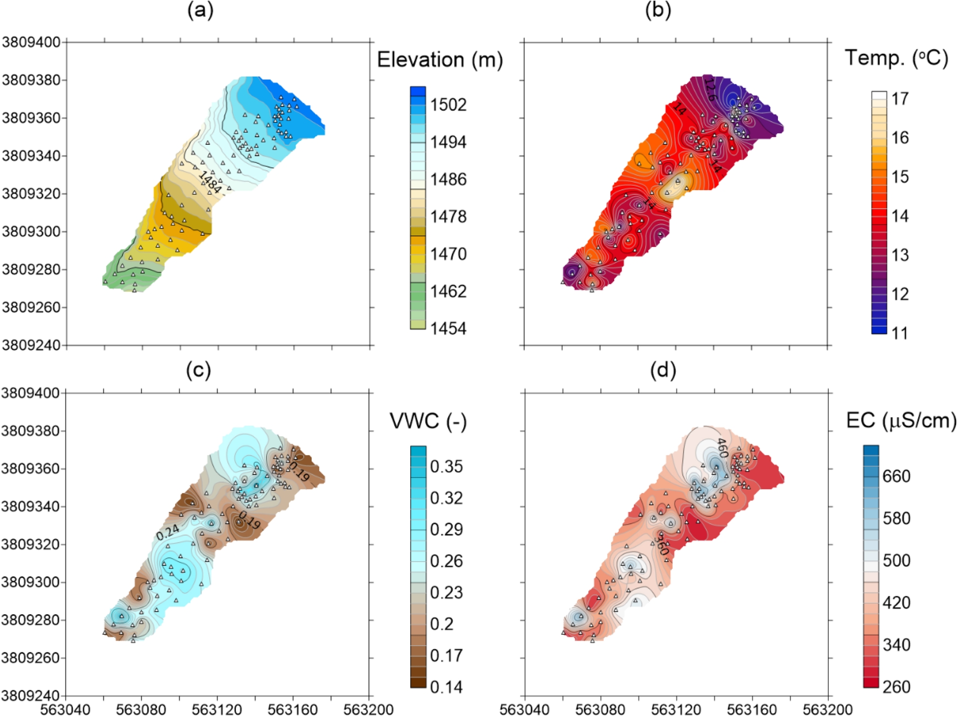
3.2. ERT results
The measured data were processed using the open-source package ResIPy (Blanchy et al., 2020) incorporating topographic modeling. Two-dimensional inversions were performed for one primary profile (L1) along the slope and three perpendicular profiles (L2–L4). The presented results have accounted for the depth of investigation (DOI). The inversion result for the profile along the slope (L1) is presented in the next section, as it was used for the SP source inversion. We also evaluated the reliability of the inversion results using the R index proposed by Oldenburg and Y. Li (1999), which indicates that the presented imaging regions are reliable except for the near-surface layer (depths shallower than ∼0.5 m). Details about the depth of investigation can be found in the Supplementary Material (Figures S7, S8).
Triangular meshing was applied during inversion, with mesh refinement around the electrode locations and near the surface, while gradually coarsening with depth (Figure 6). The resistivity model is defined on this mesh, where resistivity values are assigned to mesh vertices and rendered using linear interpolation within each triangular element. The resistivity images show a general decrease in resistivity with depth along all profiles. A pronounced transition from relatively high to low resistivity is observed at shallow depths, which is interpreted as reflecting the contrast between the unsaturated near-surface materials and deeper, more conductive zones associated with increased moisture content. This transition is inferred to indicate the approximate position of the shallow groundwater table, occurring at depths of roughly 2–5 m below the ground surface. This interpretation is consistent with the recorded water level data (Figure 4d). Overall, the groundwater level rises from the slope toe toward the head.
ERT inversion results for horizontal survey lines on (a) L4, (b) L3, and (c) L2, respectively. The white triangles represent the inversion mesh.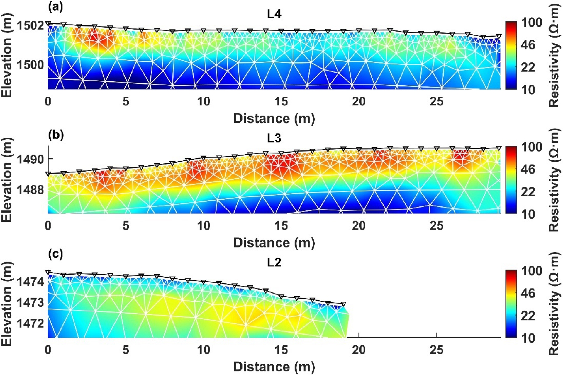
3.3. SP results
The reference potential was fixed at the slope toe, with all SP values corrected for electrode drift and temperature (Figure 7). Overall, SP values are negative, indicating a groundwater flow trend toward the slope toe (Figure 7a). The lowest SP values are found in the upper-middle section of the slope (Zone 3) beneath the residential houses (Figure 2a). SP gradients show stronger north–south than east–west variations, with a maximum spatial gradient below 3 mV/m (Figure 7b,c). Negative SP anomalies cluster in Zones 3 and 4, where 42 SP electrodes were concentrated. These areas also coincide with higher soil conductivity and steeper SP gradients (Figures 5d, 7b,c), implying stronger streaming currents and higher groundwater velocities (Equation (1)).
SP profiles: (a) SP profile corrected for temperature drift; (b) east–west SP gradient; (c) north–south SP gradient. Colored triangles indicate SP electrodes in different zones, while dashed grey lines denote the boundaries between those zones. The area enclosed by the blue line represents the high-conductivity zone.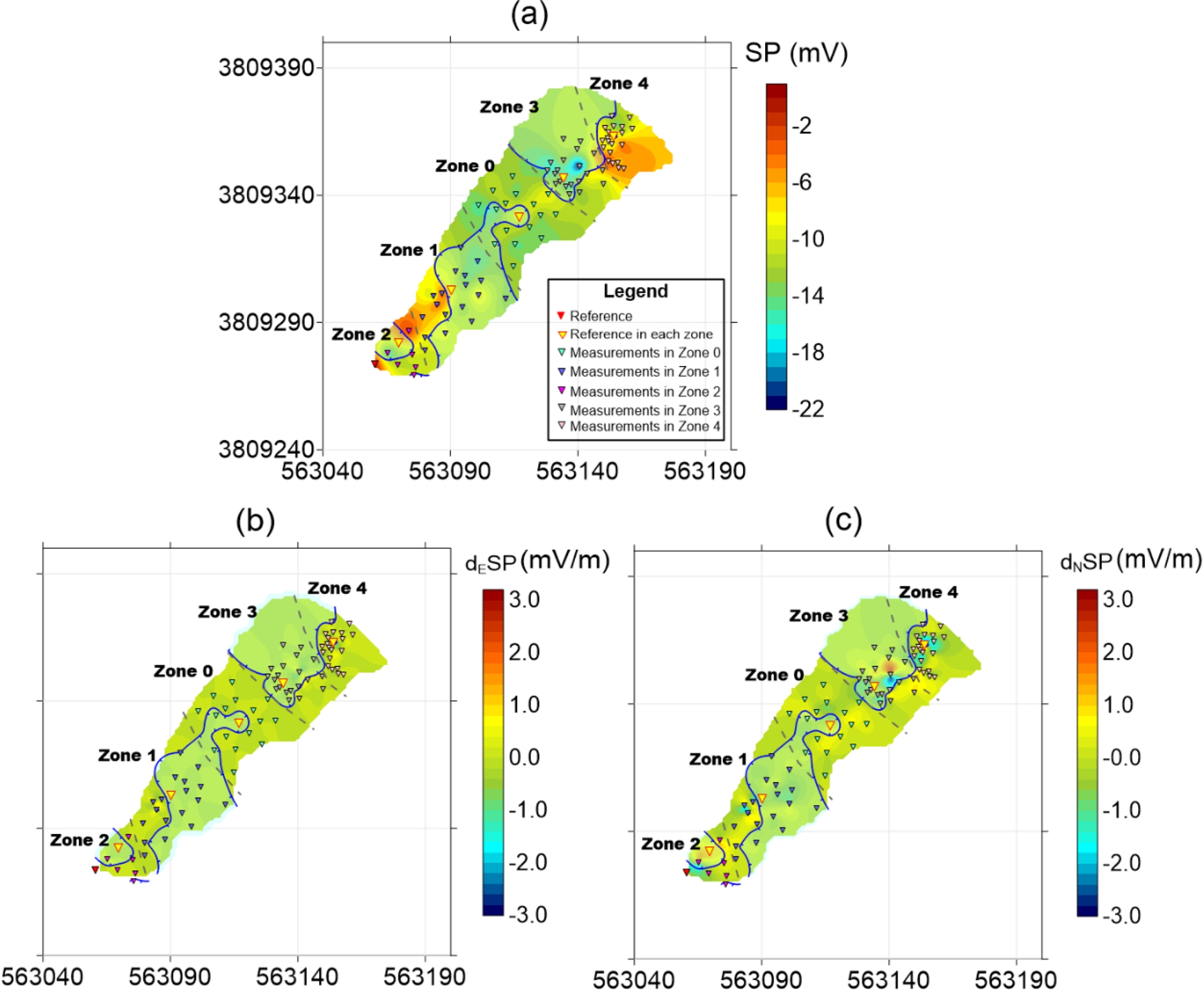
For quantitative interpretation, we performed SP inversion along L1. The final inversion (85 iterations) achieved an RMS misfit of 0.0032 mV (Figure 8). Along the L1 profile, the average SP value is −10.4 mV, with two notable negative anomalies (Figure 9a). The SP gradient, driven by electrokinetic effects, aligns with the expected groundwater flow direction. Negative SP anomalies are typically associated with infiltration and downward water flux (e.g., Bogoslovsky and Ogilvy, 1977; Zlotnicki et al., 1998). A minimum SP value (∼−22 mV) occurs at ∼92 m near the main scarp, coinciding with a sink zone identified from the SP inversion (Zone S1 in Figure 9b). This location also corresponds to the shallow conductive anomaly C1 (Figure 9c). A secondary SP anomaly appears toward the southwestern end of the profile (∼30 m), associated with another localized streaming sink feature (Zone S2). However, interpretation in this sector remains less certain, as the inversion results are affected by reduced ERT coverage and potential boundary effects.
Convergence curve of the SP inversion showing RMS misfit reduction during IRLS iterations.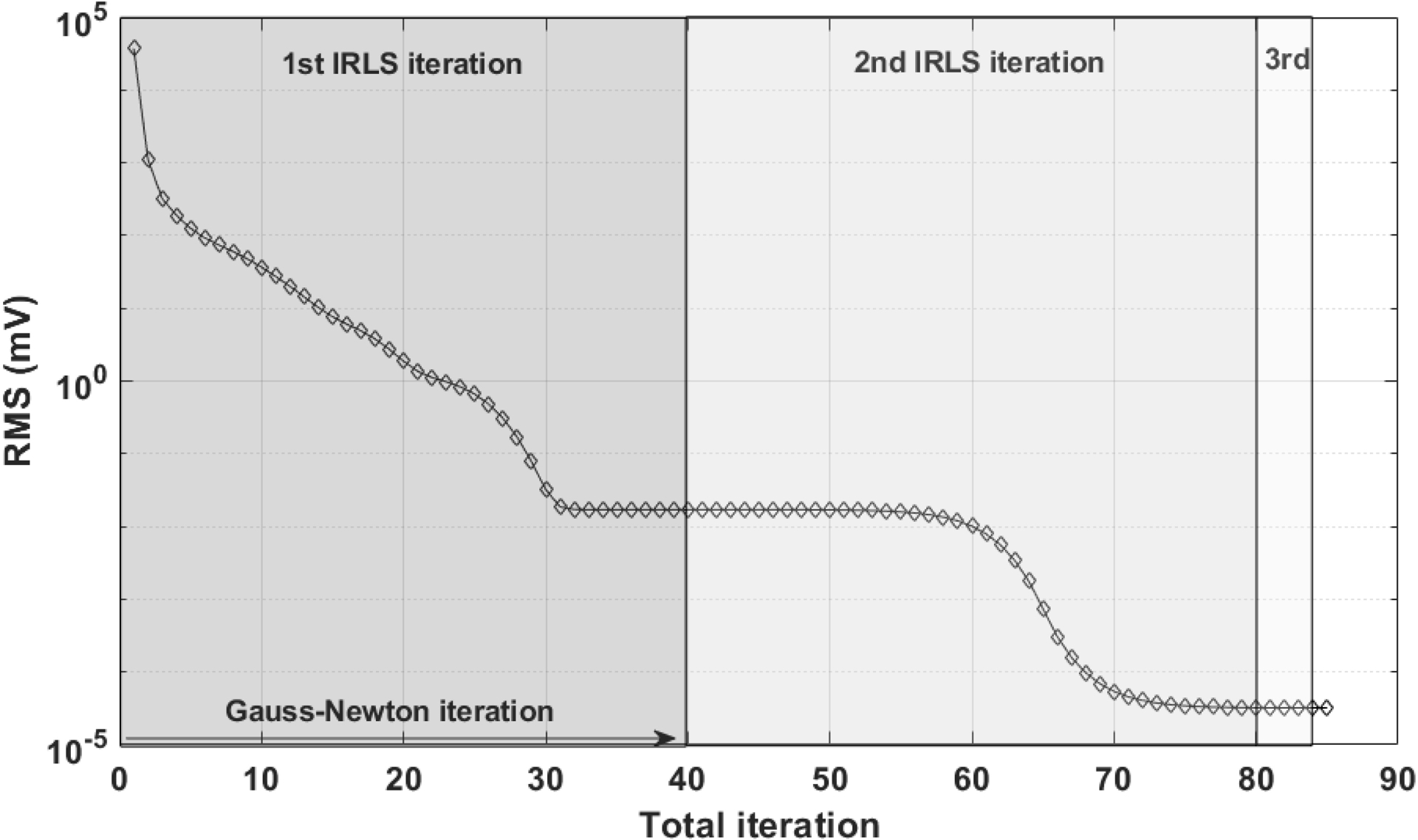
SP inversion along the survey line L1. (a) SP data and elevation of observations; (b) inverted streaming source distribution; (c) corresponding ERT conductivity model. Major negative SP anomalies (Zones S1 and S2) align with streaming sinks and conductive anomalies (Zone C1). Dashed white line denotes the proposed water level from ERT results.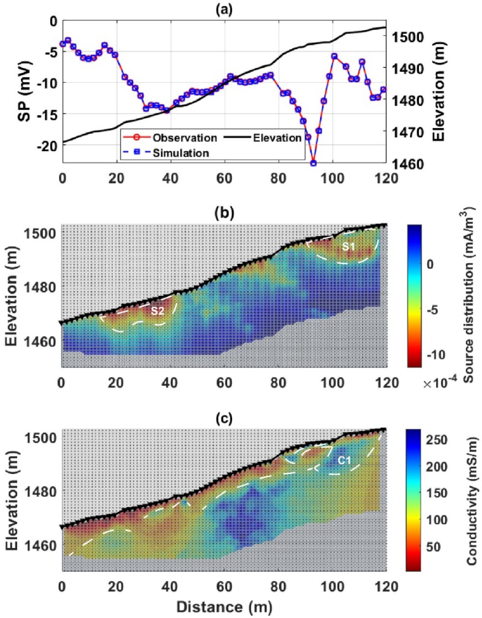
4. Discussions
Overall, the SP measurements reveal a general gradient directed toward the slope toe (Figure 7). The near-surface water content and electrical conductivity exhibit a trend of higher values in the middle and lower portions, decreasing toward the edge of the sliding mass. This spatial variation in soil properties is consistent with the topographic features of the slope. Notably, areas with high gradients in SP, water content, and electrical conductivity tomography coincide with zones of intense deformation (Figures 5c,d and Figure 7).
A particularly weak SP signal is observed within the vegetable plot ① (Figure 10), which may be partly influenced by plant transpiration, a process known to generate localized electrical potentials (e.g., Hu, Loiseau, et al., 2025). In addition, two irrigation water storage containers ④, located above the vegetable plot, likely enhance local water infiltration. By analyzing SP gradients, we inferred potential seepage pathways (Figure 10). These suggest that groundwater flows not only along the slope toward the gullies but also migrates along preferential subsurface flow channels.
The DEM covered with SP data (contour map) and areas with slopes exceeding 30 degrees (red polygons) to indicate the scarps caused by the landslide. The dashed line arrows indicate the proposed groundwater flow pathways.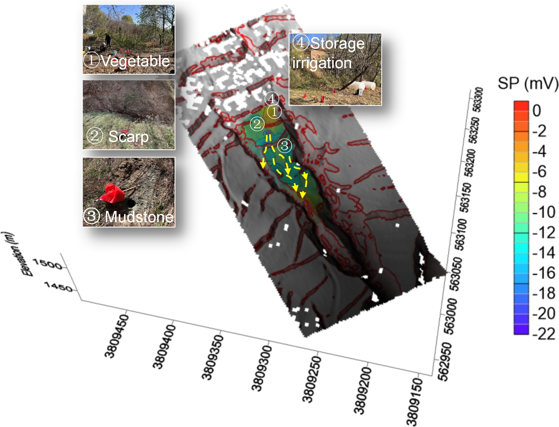
The negative SP anomaly in this area, expressed as a downward gradient, indicates active groundwater migration downslope, thereby contributing to landslide dynamics. In contrast, the low-permeability and high-conductivity mudstone layer in the central sector ③ acts as a barrier (Figures 9c and 10), impeding groundwater movement and creating spatial heterogeneity in the hydrogeological response of the landslide body.
The distribution of negative source terms also highlights potential seepage inlets (e.g., Guo et al., 2022). For example, scarp ② near Zone S1 appears to facilitate vertical infiltration, which is subsequently redirected underground to form a preferential flow channel (Zone C1). Because the subsurface consists of loess and clay, zones of high conductivity partly reflect surface conductivity and pore-water salinity effects, rather than being solely controlled by water content (Revil, Cathles III, et al., 1998). When considered together, the co-location of negative SP anomalies (Figures 7a and 9a), the sink area (Zone S1 in Figure 9b), elevated near-surface water content and reduced soil temperature (Figure 5b–c), and the shallow high conductive anomaly (Figure 5d and Zone C1 in Figure 9c) supports the interpretation of a preferential seepage pathway emerging near the scarp.
Nevertheless, SP is a potential-field method, which inherently limits the depth resolution and the ability to uniquely constrain the depth extent of subsurface sources. In addition, to account for topography and the underlying bedrock, the modeling domain was extended from the air layer down to the basal boundary (Figure 9b). This domain extension may introduce additional uncertainty in the recovered source magnitudes and affect the quantitative accuracy of the inversion results. The absence of borehole data within the study area limits vertical constraints on the electrical conductivity structure and the depth distribution of streaming current sources. Moreover, the effective excess charge density that controls electrokinetic coupling depends on factors such as pore size distribution, water content, and pore-water chemistry (e.g., Linde et al., 2007; Revil, Linde, et al., 2007; Jougnot, Mendieta, et al., 2019; Jougnot, Roubinet, et al., 2020; Hu, Jougnot, et al., 2020; Hu, Q. Huang, Han, Y. Zhang, et al., 2025; Solazzi et al., 2022), and thus likely varies spatially across the landslide body. A full quantification of Darcy flux would require specific assumptions regarding both the electrokinetic coupling coefficient and the excess charge density (e.g., Minsley et al., 2007). Therefore, while our results allow us to infer groundwater flow pathways, they cannot yet provide absolute flow rates.
To improve the understanding of subsurface water dynamics and enhance the resolution of streaming current analyses, future work should integrate SP monitoring with complementary methods such as time-lapse ERT and induced polarization, along with borehole investigations (e.g., clay content, electrokinetic coupling coefficient, permeability) and provide improved vertical resolution. Combining these approaches would enable a more robust characterization of subsurface structures and groundwater flow pathways over time.
5. Conclusion
This study employed a geoelectrical framework to investigate the Fengjiaping Landslide, integrating SP measurements with ERT to infer subsurface water pathways and identify zones potentially related to slope reactivation. The ERT results provided conductivity models that suggest the presence of a shallow water table and delineate possible aquifer distributions within the study area. The joint interpretation of SP and ERT data along the slope revealed negative SP source anomalies concentrated beneath the main scarps in the accumulation zone. These anomalies, together with cracks and scarps, likely act as preferential pathways for infiltration. The inferred coexistence of shallow water-enriched zones and clay-rich deposits appears to play a key role in governing slope instability.
Nonetheless, several limitations remain. The interpolation of SP data onto ERT electrode positions may introduce local uncertainties, particularly in sparsely covered sectors. Inversion results, especially near profile edges, are less constrained due to boundary effects and limited resistivity sensitivity. Furthermore, the adopted inversion framework assumes simplified source–flow relationships, which may not fully capture the complex, coupled hydrogeophysical processes in heterogeneous and deforming slopes.
Future work should focus on integrating time-lapse SP and ERT monitoring with complementary methods, such as induced polarization and borehole investigations, to improve vertical resolution and help constrain key parameters, including clay content, permeability, and electrokinetic coupling coefficients. Applying this integrated framework to other landslide-prone regions may enhance our ability to map preferential flow pathways and support the development of early-warning and mitigation strategies.
Acknowledgements
This work has been partly supported by the National Natural Science Foundation of China (42574089), the Postdoctoral Fellowship Program of China Postdoctoral Science Foundation (GZC20241598, 2024M753016), the China Postdoctoral Science Foundation–Hubei Joint Support Program (2025T045HB), the “CUG Scholar” Scientific Research Funds at China University of Geosciences (Wuhan) (Project No. 2023139), and the Geological Disaster Prevention Special Fund of the Gansu Provincial Department of Natural Resources (Grant No. 20230209GYY). The authors thank Dr. Jing Xie at Central South University and Dr. Wenwu Tang at East China University of Technology for discussions on the SP inversions. The dataset collected during the study have been made publicly available on the Hydrogeophysics Community of Zenodo at https://doi.org/10.5281/zenodo.17010708. The authors thank the editor and two anonymous reviewers for their comments and recommendations, which help us to improve this manuscript.
Declaration of interests
The authors do not work for, advise, own shares in, or receive funds from any organization that could benefit from this article, and have declared no affiliations other than their research organizations.
Supplementary materials
Supporting information for this article is available on the journal’s website under https://doi.org/10.5802/crgeos.327 or from the author.