

1 Introduction
More than twenty years ago, the complete sequence of the DNA of bacteriophage λ was published. Since, longer and longer sequences were deciphered, including those of such higher organisms as drosophila and man. My impression is that a world of important concepts could have been derived from a thorough analysis of simple genomes, and that instead one is engaged in a race for establishing more and more long sequences. The accumulation of data is terrifying, and the situation is reminiscent of Ionesco’s play Amédée ou comment s’en débarrasser ? A major problem now is to integrate knowledge and to try understanding more, rather than knowing more. It is fine to have a list of the elements of a system, but even more to know which elements are essential and how they interact.
In this paper, I will briefly discuss some conceptual tools that might help in this task. I will deal only with tools of which I have a direct knowledge, namely those involved in the understanding of the global operation of complex systems. This means that I will not deal at all with such extremely important items as the research of sequence homologies etc., of which I have no personal experience.
2 Circuits, the wheels of regulatory processes
Interactions between the elements of a system are commonly represented by arrows. These arrows refer to very different processes according to the case. An arrow A→+B can mean that substance A is converted into substance B, but as well that it activates the synthesis of B, etc. What is common to these diverse modalities is that A takes part in the production of B, exerts a positive action on the synthesis of B, whatever the detailed mechanism.
A→-B means that A exerts on the contrary a negative action on B, because it prevents its synthesis or promotes its decay, or... In biochemical and physiological books or papers, one finds very often long chains of interactions in which A exerts an action on B via a number of intermediate substances. However, for many purposes, in spite of the interest of the detailed pathway, the important point for the general operation of the system is whether A eventually exerts a positive or a negative action on B. This depends only on the parity of the number of negative interactions in the chain. If even, the effect of A on B is positive; if odd, it is negative. This already provides a way to integrate abundant data, just by provisionally compacting them into shorter chains, carefully taking into account the global signs.
Surprisingly, if cascades of elements are very frequent in biochemical descriptions, one finds quite seldom closed chains of interactions (‘circuits’), with the notable exception of the Krebs cycle. Yet, as we will see, circuits are so essential to the dynamics of systems, that even the fundamental possibility of having defined steady state(s) requires their presence.
The concept of feedback circuits’ (for short, circuits) was developed long ago by ecologists and biologists as closed sets of oriented interactions—the word ‘feedback loop’ is more frequently used by biologists; we prefer use ‘feedback circuit’, because in graph theory ‘loop’ is only used for one-element circuits. If x1 acts on x2, which acts on x3, which in turn acts on x1, one says that there is a circuit x1 → x2 → x3 → x1. In a circuit, each element exerts a direct action on the next element, but also an indirect action on the other elements, including itself. More concretely, the present level of an element exerts, via the other elements of the circuit, an influence on the rate of production of this element, and hence on its future level.
There are two types of feedback circuits. Either each element of a circuit exerts a positive action (activation) on its own future evolution, or each element exerts a negative action (repression) on this evolution. Accordingly, one speaks of a positive or of a negative circuit, respectively. Whether a circuit is positive or negative depends simply on the parity of the number of negative interactions in the circuit: a circuit with an even number of negative interactions is positive, while if this number is odd the circuit is negative. We call ‘n-circuit’ a circuit of n elements, whatever its sign.
The properties of the two types of feedback circuits are strikingly different. As a matter of fact, they are responsible, respectively, for two types of regulation. A negative circuit can function like a thermostat and generate homeostasis, with or without oscillations. Positive circuits can force a system to choose lastingly between two or more states of regime; they generate multistationarity (or multistability). This contrasted behaviour of the two types of circuits can be justified without any difficulty if one formalises the systems in terms of ordinary differential equations or by ‘logical’ methods 〚1, 2〛.
We just mentioned that positive circuits are involved in multistationarity and negative circuits in homeostasis. However, it has progressively become apparent that one can be much more precise. It was conjectured by Thomas 〚3〛 that (i) a positive circuit is a necessary condition for multistationarity and (ii) a negative circuit is a necessary condition for stable periodicity. These statements were further analysed and subjected to formal demonstrations 〚4–6〛; see also 〚7, 8〛.
We would like to stress here that, rather than considering each one of the elements of a circuit as a separate entity, we prefer to see it as a part of the circuits to which it may belong. To use a metaphor, rather than analysing separately each individual tooth of clockwork, we prefer to reason at the level of the wheels that carry these teeth. This does not mean that we consider the circuits themselves as isolated entities. Rather, we consider explicitly the interactions between different circuits in the same spirit as we did when analysing the interactions between the elements of each circuit.
The description just given is purely verbal, not to say somewhat vague. It is fortunately possible to define circuits in a much more rigorous way (see for example 〚4, 8, 9〛). The idea of describing the interactions in complex systems in terms of the signs of the terms of the Jacobian matrix had been described already long ago by the economists Quirck and Ruppert 〚10〛, without, however, explicit reference to feedback circuits, and by May 〚11〛 and Tyson 〚12〛.
Consider the Jacobian matrix of a system of ordinary differential equations (ODE’s). If term aij = (∂fi/∂xj) is non-zero, it means that the variations of variable j influence the time derivative of variable i. In this case, we say for short that variable j acts on variable i and we write: xj → xi. This action is defined as positive or negative according to the sign of aij. Consider now a sequence of non-zero terms of the Jacobian matrix, such as a13, a21, a32, in which the i (row) indices 1, 2, 3 and the j (column) indices 3, 1, 2 are circular permutations of each other. Non-zero a13 means x3 → x1, non-zero a21 means x1 → x2 and non-zero a32 means x2 → x3; thus, we have the three-element circuit x1 → x2 → x3 → x1. In this way, all the circuits that are present in a system can be read on its Jacobian matrix. Fig. 1 shows the circuits that are possible for a three-variable system.

The circuits in three-variable systems.
Note that the matricial and graph descriptions of circuits are dual of each other: a non-zero element of the matrix corresponds to an arrow (not a vertex) of the graph. The circuit itself can be symbolised either by the graph or by the product of the relevant terms of the matrix.
Unions of disjoint circuits are sets of circuits that fail to share any variable. For example, if terms a12, a21 and a33 are non-zero, we have two disjoint circuits: a two-element circuit between variables x1 and x2 and a one-element circuit involving variable x3. A general and elegant definition suggested by M. Cahen (personal communication) applies both to circuits and unions of disjoint circuits. A circuit or union of disjoint circuits can be identified by the existence of a set of non-zero terms of the matrix, such that the sets of their i (row) and j (column) indices are equal. The equality of the two sets of indices can be checked, for example, for the sets of terms: a12 a23 a31 (a three-element circuit), a12 a21 (a two-element circuit), a11 (a one-element circuit), or a12 a21 a33 (a union of two disjoint circuits).
Those circuits and unions of disjoint circuits that involve all the variables of the system play a special role in the generation of steady states. For this reason, we show them here (Fig. 2) in the case of three-variable systems. For the sake of brevity, we will call them full circuits, irrespective of whether they are circuits or unions of disjoint circuits. In fact, there is a very simple algorithm for extracting all the full circuits from the Jacobian matrix: it simply consists of computing the analytical form of the determinant of the Jacobian matrix. This determinant is a sum of products, of which each one corresponds to one of the ‘full circuits’ of the system. For example, for a two-variable system, the determinant of the Jacobian matrix is (a11 a22 – a12 a21) and the two full circuits are the two-element circuits symbolised by the product a12 a21 and the union of two one-element circuits symbolised by the product a11 a22.
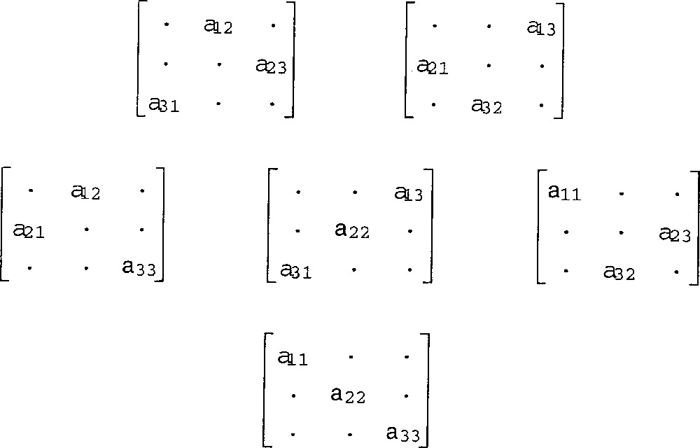
The full-circuits (circuits or unions of disjoint circuits involving all the variables of a system) in three-variable systems.
Note that a system that has no full circuit has no isolated steady state (see also 〚8, 10〛). For example, the three-variable system:
3 The relation between circuits and steady states
All the circuits of a system (and not only the ‘full circuits’) are present in the analytic expression of the characteristic equation of the Jacobian matrix. Conversely, by definition of the characteristic equation of a matrix, it is easy to see that only those terms of the Jacobian matrix that belong to a circuit are found in its characteristic equation. The terms that do not take part in a circuit belong to products that vanish, because they contain one or more zero terms. Thus, the coefficients of the characteristic equation depend explicitly only on the circuits of the system.
The off-circuit terms of the Jacobian matrix provide a one-directional connection between otherwise disjoint circuits; as a result, they may influence the steady-state values of the variables. Although they are not present in the Jacobian matrix, constant terms in the ODE’s also influence the location of the steady states. Thus, both off-circuit terms of the Jacobian matrix and constant terms in the ODE’s may play a role in the system’s dynamics. However, their role is only indirect via their effect on the location of the steady states: we would like to emphasise the fact that the eigenvalues of the Jacobian matrix at any given location in phase space depend only on those terms that belong to one or more circuit.
How the coefficients of the characteristic equation determine the stability properties of steady states has been studied for many years. Our main contribution is the recognition of the fact that all the circuits of a system, and only them, are present in the characteristic equation, as products of elements of the Jacobian matrix. This provides a basis for the notion that there is a tight relation between the ‘logical structure’ of a system (i.e., its feedback circuits) and the stability properties of its steady states (for more information on this subject, see Thomas and Kaufman 〚13〛).
4 Circuits and non-trivial behaviour
After showing that positive circuits are necessary conditions for multistationarity, and that negative circuits are necessary conditions for lasting oscillations, it was natural to try identifying which constraints on the circuits have to be fulfilled in order to have a chaotic dynamics. As far as we can tell from many examples, one needs two or more periodicities that are coupled, yet distinct in this sense that they evolve around distinct steady states. For this, one needs a positive circuit to ensure (if only partial) multistationarity and a negative circuit to generate lasting oscillations.
Here follows a qualitative analysis of a very simple three-element system that displays a chaotic dynamics (see Fig. 3):

Chaotic attractor generated by system (1) for a = 0.54. Stereoscopic view: look at the couple of images from 50 cm or so with ample lighting. Squeeze slightly in order to see a third image between the two ‘real’ images. Once you have succeeded in focusing on the third image, you see clearly the trajectory in three dimensions.
The Jacobian matrix (a positive) displays a positive 3-circuit that accounts for multistationarity and a negative 2-circuit that accounts for the oscillations. Let us reason in terms of full-circuits. One can see that they are two:
- • (I) if isolated, the positive 3-circuit would generate a saddle focus of type +/– –;
- • (II) if isolated, the union of a negative 2-circuit in xz (destabilised by the positive diagonal term in x) and of a negative 1-circuit in y, would generate a saddle-focus of type –/+ +.
In view of the odd character of the non-linearity used (x3), there are three steady states, two of which, (–1, 1, –0.5) and (1, –1, 0.5), symmetrical vs the ‘trivial’ one (0, 0, 0). But which one of the steady states will be of type +/– –, which one of type –/+ +? (In our notation, +/– – means that there is one real, positive, eigenvalue and a pair of complex conjugated eigenvalues with negative real parts, etc.) A look at the Jacobian matrix shows that, at the trivial steady state, full circuit II is non-existent. This steady state is thus expected to be generated by full circuit I, and thus to be of type +/– –. It is indeed the case, as shown by the eigenvalues (+1, –0.75 ± 0.66 i). In contrast, at the two other steady states, the product representative of full circuit II is dominant and the steady states are both of type –/+ +. As a matter of fact, they have the same eigenvalues: (–0.74, +0.12 ± 1.63 i) for obvious reasons of symmetry.
This system was chosen (and in fact synthesised) in order to show that the two distinct periodicities required for a chaotic dynamics can be generated by the same negative circuit (here, the negative 2-circuit in xz). This is the reason why we have used x3 as the non-linearity: the corresponding term of the Jacobian matrix is 3 x2, which is always positive. If we had used, for example, x2 instead of x3, the corresponding term of the Jacobian matrix would have been 2 x, whose sign depends on the sign of x, and the 2-circuit would have been positive or negative, depending on the sign of x. (This would not have prevented the system from displaying a chaotic dynamics for appropriate parameter values, but it would not have been possible to show that a single negative circuit can be sufficient.)
In the example just described, we have avoided the use of an ambiguous circuit in order to better unravel the respective roles of the positive and negative circuits. In contrast, we will now exploit the properties of ambiguous circuits as follows. Since in non-linear systems a circuit can be positive or negative according to its location in phase space, it was tempting to check whether a system with a single circuit can generate chaos, provided it is ambiguous. It was found to be indeed the case 〚14〛.
Finally, we would like to show here a case in which the mere inspection of the signs of the interactions gives precious information about the dynamical possibilities of the system. Consider the matrix:
This matrix comprises three full-circuits: a negative 3-circuit, the union of a negative 2-circuit in xy and of a negative 1-circuit in z and the union of three 1-circuits (the diagonal terms). This indicates the possibility of three types of steady states: a saddle focus of type –/+ +, a steady state of type – – – or – / – – depending on the parameter values, and a stable node (– – –). However, the absence of any individual positive circuit precludes any multistationarity. Consequently, in this system, one can have either of theses three types of steady states, depending on parameter values, but they cannot coexist.
5 Logical description of dynamical systems
Complex systems almost invariably comprise non-linear interactions. This is not only the case in biology, but in other fields too, like economics, and probably in general. In fact, the presence of non-linearities is an essential ingredient of so-called ‘non-trivial behaviour’, such as multistationarity, stable periodicity or deterministic chaos 〚15〛.
This complicates the analysis of the behaviour of systems, because in general systems of non-linear differential equations have no analytical solution. In order to simplify the treatment, one may be tempted to idealise the description. The most obvious idealisation is the linear ‘caricature’. It is well known that this idealisation is disastrous, except in close vicinity of a steady state, which in addition has to be unique. In practice, the non-linear interactions very often display a sigmoid shape. For example, the fixation of oxygen by haemoglobin is insignificant for low partial pressures of the gas; it increases rapidly within a rather narrow range of the pressure, and soon saturates for higher values. The shape of the interactions can be described by the well-known ‘Hill function’, but as well by the hyperbolic tangent. More generally, sigmoids can be described as curves with two horizontal boundaries and a single inflection point. It is tempting to caricature steep sigmoids by step functions, and this is why it has been repeatedly proposed to use a logical description of systems comprising sigmoid interactions. In spite of its apparent brutality, the assimilation of (sufficiently steep) sigmoids to step functions keeps all the essential features of the dynamics, including the number and nature of the steady states (see the beautiful papers by Glass and Kauffman 〚16, 17〛, and also Kaufman and Thomas 〚18〛). It is often objected that in biochemistry and elsewhere not all interactions are sigmoid and that many of them are linear. As a matter of fact, it was realised that sigmoids ‘compose’ (except in quite ‘pathological’ cases), that is, if F1(x), F2(x) and F3(x) are sigmoids, F1(F2(F3(x))) itself has a sigmoid shape as defined above (Reignier et al., in preparation). They compose also with linear functions. The resultant sigmoid is increasing or decreasing, depending on whether an even or an odd number of decreasing sigmoids is involved in the composition, and the steepness of the resultant curve increases with the number of sigmoids involved. It results that a chain comprising not only sigmoids but also linear interactions can be caricatured by a step function, provided the resultant sigmoid is sufficiently steep. Using step functions amounts to reason as if an element was absent below a certain threshold and present above this threshold.
6 Logical description: asynchronous vs synchronous
In the logical description of systems, to each relevant element is ascribed a logical variable that has only two values (0 or 1) in simple cases. The state of a system can thus be described as a logical vector. Classically, time is included in the description by giving the state vector at time t + l as a function of the state vector at time t. In this so-called ‘synchronous’ description, each state has one, and only one possible successor, without any possibility of choice. In addition, if a state and its successor differ by the values of more than one variable, the description implies that the values of two or more variables change in exact simultaneity, a quite unrealistic issue. For example, in the system
| 1 |
For this type of reasons, instead of comparing the state at time t with the state at time t + l, we consider (at any time) a state and its image for the logical functions of the system. Thus, instead of writing (1), we write:
Here, the image of state 00 is 11, but this does not mean that the next state of 00 will be 11. Rather, variables x and y have both a command to switch from 0 to 1, but there in no reason whatsoever for these commands to be executed simultaneously; if variable x switches first, the sequence is 00 → 10; if variable y switches first, the sequence is 00 → 01. Thus, from state 00, the system can proceed to states 10 or 01; the exactly simultaneous change of both variables is not excluded, but considered marginal. In our description, the choice between the transition 00 → 10 and the transition 00 → 01 depends on the relative lengths of two time delays tx and ty, and on the choice between the transitions 11 → 0 1 and 11 → 10 on the time delays and
This is the ‘asynchronous’ description, of which the synchronous description is a particular, marginal, case. In spite of a superficial similarity, the synchronous and asynchronous descriptions are deeply different, and give extremely different predictions. Without entering into details, let us mention that the elaborate versions of the asynchronous description fit admirably with the differential description (provided the interactions involved in the ODE’s are step functions or sufficiently steep sigmoids), whereas the synchronous description predicts artefactual attractors.
7 Generalised logical description
It was felt obvious from the beginning that a purely Boolean description, using 0 and 1 as the only possible values for the logical variables, would be too primitive in many cases. A first improvement consisted of using ‘multivaluate’ logical variables whenever required. In agreement with the views of Van Ham 〚19〛, we do not use multivaluate variables systematically to improve the resolution of the description. Rather, we use them only when there is a qualitative reason for it. In fact, whenever a variable acts on more than one function, the threshold above which it is active may be different according to the function considered. Consequently, when a variable acts on n functions, we associate up to n thresholds to this variable, which can thus have up to n + 1 logical levels. This can be formalised with a multivaluate variable or an appropriate set of Boolean variables.
Another crucial, additional sophistication was ensured by the introduction of logical parameters by Snoussi 〚1, 2, 20〛. For short, to each interaction i can be ascribed a characteristic weight, described by a real value Ki. This leads to ‘semi-logical’ functions comprising both Boolean variables and real parameters. These functions are subject to operators of discretisation, which convert their real values into discrete values, according to a scale characteristic of each variable. Without entering into details, state tables now contain logical parameters K, each of which can take any of the logical values permitted to the corresponding variable. Depending on the values ascribed to the logical parameters, one has several state tables, which correspond to a variety of dynamical behaviour. This results in a considerable extension both of the subtlety and of the generality of the description.
Classically, logical descriptions fail to recognise those steady states located on one or more threshold value. The simple reason is that when a real variable x is discretised into a logical variable x, one states that x = 0 if x is below a threshold value, x = 1 if x is above this threshold value, but the limit case x = 0 is not considered. In order to be able to identify all steady states (and in particular unstable steady states) in logical terms, one has to introduce the threshold values into the scale of the logical values. The scale 0, 1, 2, ... thus becomes 0, sl, 1, s2, 2, ... and we have to distinguish regular states, in which all the variables have integer values, from ‘singular’ states, in which one or more variable is located on a threshold. We call characteristic state of a circuit (or union of disjoint circuit) the state located at the thresholds involved in the circuit. For example, if x, above its second threshold, influences the production of y, which, above its third threshold, influences z, which in turn, above its first threshold, influences x, the characteristic state of the circuit is s2 s3 s1.
At first view, one might fear that the logical description has lost its genuine simplicity, if only because the number of conceivable states of the system has become considerable. However, as described by Thomas 〚2〛 and shown by Snoussi and Thomas 〚21〛, only those states that are characteristic of a circuit (or union of disjoint circuits) can be steady and, reciprocally, if a state is characteristic of a circuit, there exist parameter values such that this state is steady.
Thus, it is not necessary to scan all the (often many) possible states of a system to check their stationarity. One can simply identify the circuits and unions of disjoint circuits, note for each of them the characteristic state, and compute the combinations of values of the logical parameters for which it is steady. In this way, the space of the logical parameters is partitioned into a finite (and often quite small) number of boxes within each of which the qualitative behaviour is uniform. This permits to have a general view of the various dynamical possibilities of a system. Once the interesting ranges of values of the logical parameters have been identified, it is always possible, if required, to build a system of differential equations (with sigmoid or step interactions) that behaves in the same qualitative way as the logical system.
8 Reverse logical approach
Even though the logical approach was initially thought of as a tool for a deductive, analytical approach, it can also be used ‘backwards’, in an inductive, synthetic way (‘reverse logic’): from facts to models rather than from model to predictions. This synthetic type of approach was used already long ago (e.g., 〚22〛) for conceiving logical machines and adapted since to our logical approach 〚1, 23–26〛.
It must be clear right away that even where the type of models considered is well defined (for example, the description of a circuit of neurones in terms of asynchronous automata), a given behaviour is usually consistent with several, or even many specific models. Essentially, one starts from an empty state-table and fills only the image values that correspond to the desiderata. The other image values are replaced by dashes, which mean that their value is undetermined; in a Boolean system, each dash of such a partial-state table can be replaced indifferently by a ‘0’ or a ‘1’ without affecting the desired behaviour. Well-established methods permit to derive the simplest systems of logical equations that fit the desiderata. Alternatively, one can compare the state table of a pre-existing model that is not entirely satisfactory with the requirements of the partial table, and modify any value of the model that would not fit the requirements.
9 To summarise
Among the tools that may help finding the essential qualitative features of complex dynamical systems, we propose the systematic identification of the (feedback) circuits that govern the behaviour of these systems. Whenever a network is described under the form of differential equations, the circuits can be identified without any ambiguity from the Jacobian matrix of the system. Once characterised, the circuits may be used as described above to short-circuit more classical approaches and yet get a global idea of the possible dynamics of the system.
As regards the logical description, it must be made clear that its scope is less general than that of the approach based on the circuits. It can be viewed as an independent method for those systems that afford being caricatured in terms of step functions. Alternatively, the logical method can be used in symbiosis with the classical description as sets of differential equations. However, a satisfactory fit between the two descriptions can be expected only if the dominant interactions are step or sigmoid in shape. For recent detailed papers on the logical method, see 〚25〛 or (in French) 〚26〛.
Acknowledgements
This work was supported by the Belgian Programme on Interuniversity Poles of Attraction and by the program ‘Actions de recherche concertées’, ARC 98-02 n° 220 launched by the Division of Scientific Research, French Community of Belgium.
Version abrégée
Dans bien des domaines, la recherche souffre d’un excès de données. Intégrer ces données est devenu un problème majeur, qui revient à comprendre davantage plutôt que de savoir davantage. Il est certes utile de connaître tous les éléments d’un système. Encore faut-il pouvoir discerner lesquels jouent un rôle crucial, et comment ceux-ci interagissent.
Nous décrivons dans ce texte trois outils conceptuels, dont l’usage s’est révélé fécond, d’abord dans le domaine des régulations biologiques, puis, plus récemment, dans le domaine plus général de la dynamique non linéaire.
1. Lorsque des variables d’un système interagissent entre elles de manière bouclée, on dit qu’elles forment un circuit de rétroaction (feedback en Anglais). Un système complexe peut comporter plusieurs, voire de nombreux circuits imbriqués ; chaque circuit garde néanmoins son identité, même si la présence d’autres circuits interfère avec son action. On distingue deux types de circuits : ou chaque élément du circuit exerce sur sa propre évolution (via les autres éléments du circuit) une action positive, ou chaque élément exerce sur sa propre évolution une action négative. Tout naturellement, on qualifie ces deux types de circuit de positifs et négatifs, respectivement. On sait maintenant que la présence d’un circuit positif est une condition nécessaire à la multistationnarité, comme la présence d’un circuit négatif l’est à une périodicité stable. Tout circuit peut être identifié et caractérisé sans ambiguïté par l’examen de la matrice jacobienne du système : en fait, si une séquence de termes de la matrice forme un circuit, les séquences des indices de ligne 〚i〛 et de colonne (j) sont des permutations circulaires l’une de l’autre. Ceux des circuits (ou unions de circuits disjoints) qui concernent toutes les variables du système jouent un rôle privilégié. Nous les appelons « circuits pleins ». La liste des circuits pleins d’un système n’est autre que la liste des éléments non nuls du déterminant de la matrice jacobienne. Dans un système non linéaire, la valeur, et même le signe, d’un élément de la matrice jacobienne peut dépendre de la localisation dans l’espace des phases. Il en est de même pour les circuits : un même circuit peut être positif ou négatif selon la localisation. On parle dans ce cas d’un circuit ambigu. Notre texte donne quelques indications sur la « circuiterie » requise pour obtenir divers processus non triviaux (multistationnarité, périodicité stable, chaos déterministe).
2. Quoique nous utilisions surtout, actuellement, la description différentielle, nous sommes convaincus qu’une description pleinement quantitative d’un système complexe gagne souvent à être préparée par une description préalable qui fasse ressortir l’« essentiel qualitatif ». Ce résultat peut être obtenu par une description logique, dans laquelle les variables ne peuvent prendre qu’un nombre limité de valeurs discrètes, à savoir deux seulement (0 ou 1) dans les cas les plus simples (description binaire, ou booléenne). Nous insistons sur le fait que cette description logique doit être asynchrone si l’on veut que le modèle puisse rendre compte d’évolutions multiples, tout en évitant les attracteurs « artefactuels ». L’emploi, lorsque cela s’avère nécessaire, de variables et de fonctions logiques à plusieurs niveaux et l’introduction, cruciale, de paramètres logiques 〚20〛 rend l’outil logique extrêmement performant. L’image est qualitativement très proche de celle que fournit la description différentielle, tout au moins lorsque les interactions principales sont de type sigmoïde ou à seuil. Dans la description continue, le balayage de l’espace des paramètres est une entreprise redoutable. Dans la description logique, chaque paramètre ne peut prendre qu’un nombre fini (et généralement petit) de valeurs. L’espace des paramètres est donc constitué d’un nombre fini de pavés, dont chacun correspond à un comportement qualitatif. L’analyse du comportement de chacun de ces pavés donne donc une image complète des comportements qualitatifs possibles au sein d’un modèle. Le plus souvent, cependant, cette analyse exhaustive peut être remplacée par l’identification, bien moins laborieuse, des conditions de fonctionnalité des différents circuits. Les conditions de fonctionnalité d’un ensemble de circuits est la simple intersection des conditions de fonctionnalité des circuits individuels considérés.
3. Le plus souvent, la démarche du concepteur consiste à élaborer un modèle par allers-retours successifs (feedback !) entre les données expérimentales et des considérations rationnelles. Il se préoccupe ensuite des prévisions du modèle, vérifie s’il rend bien compte des données connues et tente d’identifier d’éventuelles prévisions intéressantes. Cette démarche fait appel, non seulement au raisonnement, mais aussi à l’intuition, et il est heureux qu’il en soit ainsi. On peut cependant rêver d’une approche qui partirait d’un ensemble de faits expérimentaux et tenterait de bâtir des modèles de manière entièrement rationnelle. Cette approche synthétique, inductive, est en quelque sorte une « logique inverse ». Un élément crucial de cette démarche est l’établissement d’une liste de contraintes qui doivent absolument être satisfaites pour que le système puisse suivre le comportement observé. Même lorsqu’on s’adresse à une classe bien délimitée de modèles (comme, par exemple, la description d’un élément du système nerveux en termes de neurones, traités chacun comme une simple variable logique, et de leurs interactions), on voit aussitôt que, dans la plupart des cas, plusieurs et, bien souvent, de nombreux modèles seront compatibles avec les données expérimentales. Se pose dès lors le problème d’identification de ceux de ces modèles qui peuvent présenter un intérêt. L’un des critères est la recherches des modèles les plus simples. Une autre approche peut consister à reconsidérer un modèle préexistant, partiellement mais incomplètement satisfaisant, et à vérifier quelles spécificités du modèle sont en contradiction avec les contraintes mises en évidence par la méthode « inverse ». Les techniques appropriées à cette démarche sont classiques.