

1 Introduction
1.1 The need for fitting surfaces to sections
It becomes common that a three-dimensional (3D) model of some of a patient's anatomy is available before a few sectional images of the same anatomical region are to be acquired again, possibly in a different imaging modality. For instance, after a patient had a C.T. scan showing a tumor, one can use sonographic sections of the same anatomic region to perform a biopsy. It can then be of interest, given a single sectional image, to locate its plane within the formerly acquired volumic dataset and perform data fusion. As the imaging modalities are different, one is often left with only the simplest clues, like organ or vessel boundaries, to perform the matching.
In this paper we describe an algorithm which, given a surface model and one of its oblique cross-sectional curves, retrieves a plane that cuts the surface along the same curve. We define the problem as of fitting the surface to one of its planar cross-sectional curves: we fix a plane with a sectional curve in it, and we want to compute a rigid transform in space that will bring the surface from a position of reference to a position where its intersection with the fixed plane coincides with the given curve.
The algorithm permits exploring to what extent the fusion of the two datasets can rely on merely recognising a surface in the 3D scene and a curve in the sectional image. As we assume the surface to be rigid, the algorithm is not always applicable to the clinical problem first mentioned. Some methods like gating or cyclic volume acquisition may however adapt it to more general cases.
We shall distinguish two parts in the problem. The local problem solves the final part of the search where the state is close enough to the solution to require only small steps, which permits using techniques of differential calculus on manifolds and a Lie group formula. We avoid using a distance function to be minimised, instead directly requiring a certain deformation to be obtained for the intersection, which we represent by a vector field along the intersection curve (Fig. 1). It is from that vector field that one computes a vector (element of a Lie algebra) tangent to a satifactory displacement of the surface, and then a true displacement using a classical closed formula for the exponential of the Lie group of rotations.
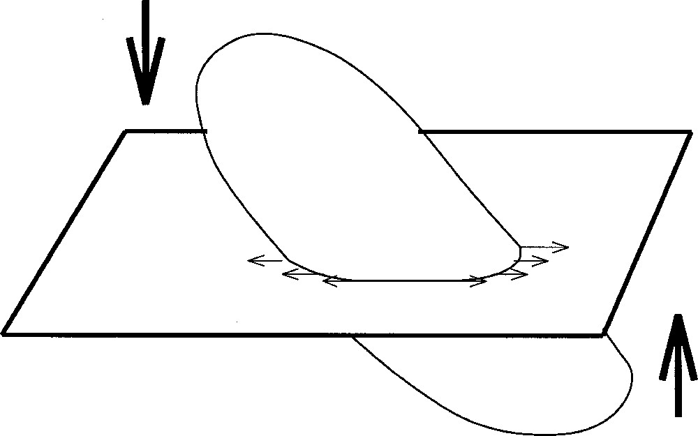
The surface, the fixed horizontal cutting plane, and the effect of a displacement of the surface on the shape and position of the sectional curve: the moves of the intersection points are accounted for by a vector field along the intersection curve. The problem addressed in this article is to find a position of the surface so as to match the intersection with a curve already given in the plane.
The global problem is that of choosing a starting position for the surface such that the local search will lead to a solution, escaping local minima. We first build a sectional atlas, i.e. a catalog of cross-sections of the model surface in different positions, then we query it, comparing the intersection for the starting position to the sections recorded in the atlas in order to find a best match and start from the corresponding position. Justifying that procedure and looking for optimised atlas calls for definitions and some formalism that we briefly outline to sketch our research prospects. The complexity of the problem calls for contemporary mathematical techniques such as genericity methods and Catastrophe Theory, which we also use to simplify the algorithmics of plane intersections.
Notice that there is in general no unicity in the solution. This is trivially true for the tangential sections of the surface, several of which are unique points obtained for different plane positions. Excluding these cases obviously still leaves the possibility of multiple solutions, but whether unicity holds generically seems to be an open problem.
1.2 Other approaches to searching: generic signs for humans
Let us put in a more general perspective this problem of searching for a position parameter (here the unknown transform) in view of a controlled image (here the target intersection curve). It is common in medical imaging to deal with families of images. For instance, a sonographic image is controlled by such parameters as the direction and position of the probe, the contrast parameters, the position and breathing of the patient. A convenient mathematical formalism is that of mapping controls 〚1, 2〛: each image is modelled by a differentiable mapping within a continuous family depending on the coordinates in a control space. Exploring a patient is then a kind of navigation in control space where one tries to obtain certain images in the family, or to prove that they are not present. Most imaging modalities involve families of projections or families of sections of surfaces, and for these a theory has been evolved from the methods of differential topology 〚3, 4〛 to show how some of the usual radiologic inferences are valid 〚2〛. Important sign systems used in medical imaging rely on genericity assumptions 〚5〛. Roughly speaking (see below), this means that there are exceptions to the rules used, but that the exceptions are so rare that reliable inference is possible.
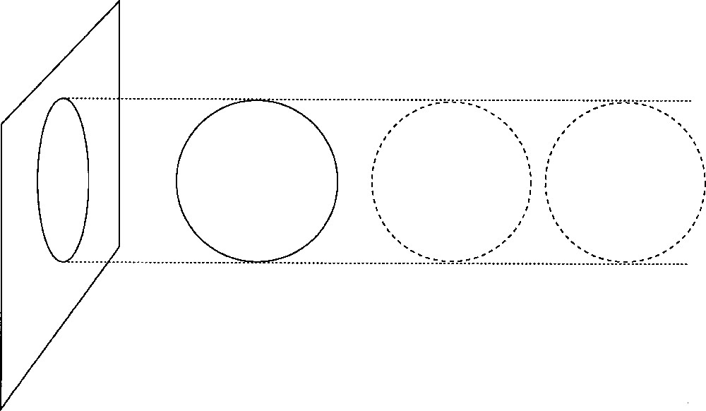
For instance, in the case of standard projection radiographs, the lines extracted by the radiologist's eyes on the image are formed on the film where the projecting X-ray hitting the film has been tangential to a contrast surface in the patient's body (a situation associated to a singularity of the projection of the surface on the film along the rays). A generic sign system for the interpretation of radiologic projection images is made of three signs: a line comes from a fold of the contrast surface, two crossing lines come from the superposition of two folds (this accounts for what is known in Radiology as the “silhouette sign”), and a cusp comes from a pleated contrast surface. Counter-examples to these rules can easily be constructed mathematically (Fig. 2), and seem to prove the impossibility of making interesting inferences about the surface from the lines on its projection, but they are unstable and rare and so do not prevent the use of the sign system in practice.
Ambiguity arises from some experimental settings, since different sets of contrast surfaces may lead to the same projection image. This seems to prevent any rigorous interpretation procedure for projection imaging. However, the ambiguous configurations are unstable (here, perturbing the surfaces would almost certainly separate their images) and rare enough to be neglected in practice, which is mathematically justified using genericity.
Such sign system is justified in the absence of a precise control on the angles of projection, but in case one precisely monitors and controls the angles it is possible to stabilise special positions and make new image patterns appear. One of them is the “swallow-tail” described in Catastrophe Theory, which can generically be stabilised (this notion of genericity takes the control into account) when observing tangentially a piece of surface with a negative curvature and turning it around an axis normal to it (Fig. 3). There is a sign system for surfaces under one-parameter control, another one for two-dimensional control. Seeing a swallow-tail pattern on an image permits predicting in practice what rotations will increase it or make it disappear.
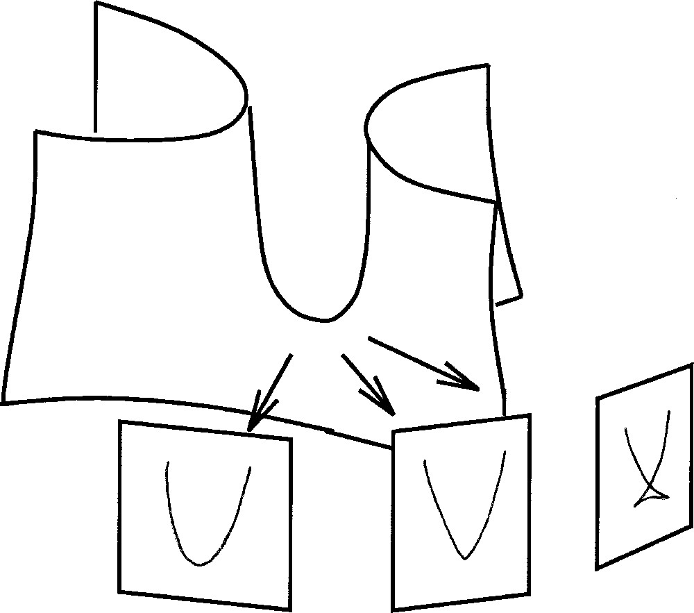
Some local signs indicate how to move the patient to modify the image in a certain way. Here a swallow-tail pattern seen on a projection of a portion of a tube (the right image displays it unfolded into a stable image combining two cusps and one crossing) indicates an axis around which to rotate the patient and cancel the pattern. In this figure, the film is equivalently rotated around the patient. The left image is also stable, the middle one (unstable) is a transition.
The problem we address in this paper is to be solved with numerical methods using computers. Let us remember however what alternative methods are used by human experts to navigate families of images: some images include special patterns that can be recognised and used to guide the search. For instance, in the case of radiograghic projections, a swallow-tail pattern generically indicates an axis around which to rotate the patient in order to either increase it or remove it (a standard clue when imaging the digestive tract, especially when examining the stomach or the colon). In the case of sectional imaging, a cross-section generically displays only regular curves, but controlling one parameter such as the level of the section generically stabilises two new patterns: an isolated point is associated to either the birth or the disappearance of a curve, and a crossing corresponds to the merging of two curves or to the splitting of a curve. Here again, one can use these signs as hints to the control when searching for certain images. For instance the crossing pattern is ‘announced’ by some ‘attraction’ of two contours, i.e. detecting that a move of the sonographic probe pulls two curves towards each other is a good clue when looking for a crossing.
In all of these instances, the search is guided by the qualitative recognition of some local or regional patterns, as opposed to the global averaging to be performed by the algorithm we are about to describe. Merging these two approaches might be proposed as a direction for future research.
2 The local problem
2.1 Setting and notations
Let us call the set of displacements in . Each element of can be described as a couple where T is a translation and R a rotation, or, using projective transforms, as a 4×4 matrix:
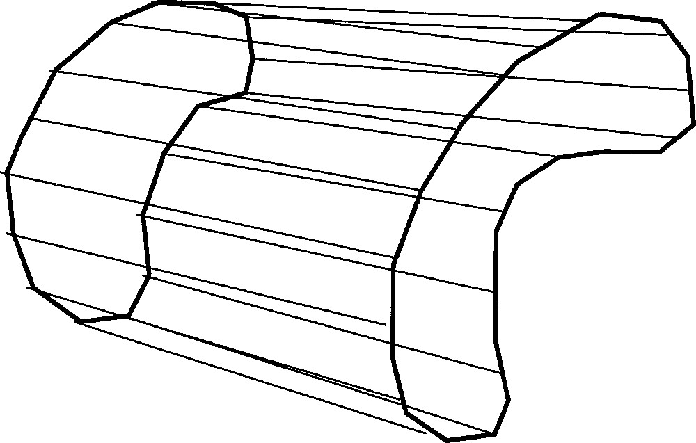
The surface S we shall consider will be a finite triangulated polyhedron coded in a standard ‘.polyh’ file format. Let us consider the plane it generically cuts only edges of S and no vertex of it. We call tube of the cross section the set of the vertices of the edges of S which are cut by P (Fig. 4). Let tub be the current tube. Of course tub is recorded within a proper data structure, e.g., to relate it to the data structure recording the cross-sectional curve To compute one needs only know the coordinates of the elements of tub. We assume these to be an element of a 6n-manifold Tubes, with n the number of vertices of CS, allowing some redondency for coding convenience. Computing CS maps Tubes to some 2n-manifold E representing the embeddings of polyhedral curves into P.
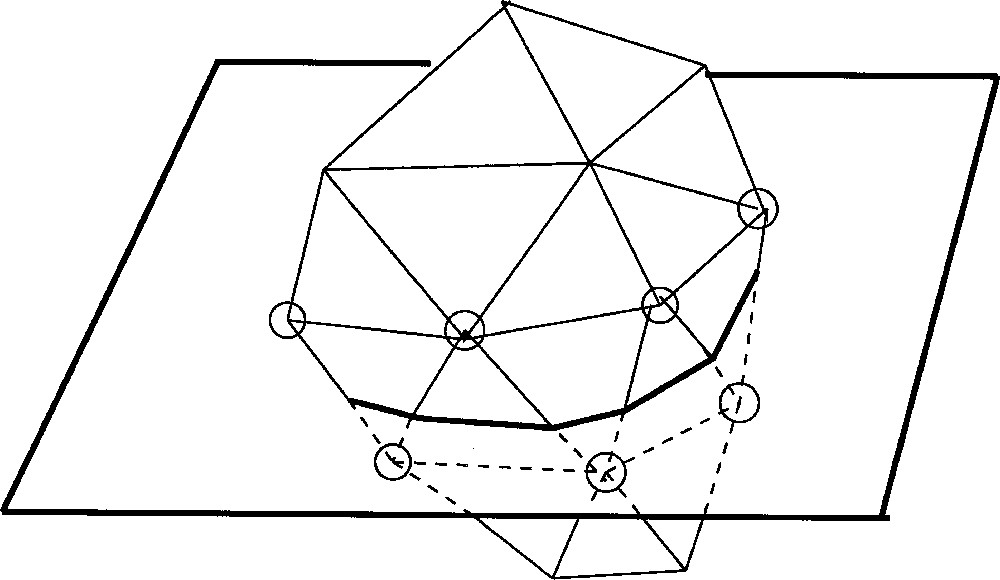
The discrete tube around the plane intersection of a triangulated polyhedral surface: knowing the circled vertices is enough to compute the intersection curve.
We shall assume here that we are given a distance function evaluating for each position of S how close CS is to the fixed target curve Ct given in P. We wish to find a position (unique or not) of S in space which minimises that distance to Ct. For the time being, we shall aim at approximating some vector field V along CS (in P) proportional to the gradient of d.
Each element of acts on S in 3-space, and thus on tub, then on CS, and eventually on
To carry an infinitesimal approach, we shall consider the tangent spaces to these spaces and compute the Jacobian Jh of the mapping h=g[j0]f from to E. This Jacobian not being invertible, we shall use a least-square approach to find an element X of generalized solution to the equation where V will be a displacement of the curve CS improving its fit to Ct. We then need to find an element of close to X to be able to perform a true displacement the effect of which on Ct will approximate V. To do so we use the Lie group structure of and an exact formula for the exponential from (its Lie algebra, a product of the space of antisymmetric 3×3 matrices and translations) to The distance from CS to Ct is iteratively decreased, taking into account some requirement of smallness of the steps so that the non-linear computations involved in the tube intersection remain well approximated by this linear approach.
2.2 Implementation
Recall that X is the element of which we are looking for. X and its transforms by and can be represented by matrices:
Matrix X is only a vector presentation of the same element of usually viewed as the matrix of a linear mapping, where is the antisymmetric matrix of the linear mapping tangent to the rotation R which is the first component of the element
The tangent mappings and have matrices:
As a consequence, the equation to be solved i.e., develops as
More precisely, the matrix we build is:
Matrix M has no inverse but equation has a generalised solution, i.e., using Euclidean norm, the minimal norm vector field among those the effect of which approximates best the required vector field 〚6〛. It is computed using standard numerical procedures 〚7, 8〛.
To find a true displacement close to the antisymmetric matrix associated to X, we use the exponential mapping from to for which there is an exact formula:
Finaly, the matrix of the transform to be performed on surface S is:
Each loop of the algorithm consists of the following steps:
- 1. 1)compute the intersection of Swith the given plane P,
- 2. 2)form matrices M, V, and find a generalized solution to ,
- 3. 3)compute the displacement and apply it to S.
At each step 1), the genericity of the intersection is checked (it is necessary for keeping simple of the intersection algorithm and the data structure for the tubes). If some vertex of the polyhedron is found in P, a small transformation is performed on the surface and the loop is resumed at the point of entry of the intersection algorithm (see below for the justification of this simple algorithm using genericity).
2.3 Choosing the vector field along the intersection
The former section showed how to compute an infinitesimal displacement of the surface that will produce a given deformation of the intersection curve. We now have to specify the required deformation. That deformation is a sort of vector field along the intersection curve, i.e. in the present case of a polyhedral surface, a mapping associating to each vertex of the intersection polygon a vector in figuring the translation to be applied to that vertex. We want the successive applications of such required vector fields to bring the intersection curve to the target curve. A vector field along a curve can be seen as a vector tangent to the space of curves at the given curve, and such tangent vector can be the gradient of a functional defined in the space of curves. Taking as the functional a distance from any curve to the target curve, following the gradient will lead a curve towards the target curve as desired, at least starting from a neighbourhood of the target curve. Some of the natural distances on the space of curves, such as geodesic distances deduced from a scalar product on vector fields along curves, are difficult to compute, and a gradient has to be output. We have some latitude in the choice of a distance, and also in the vector field, which only needs to contribute a decrease in distance, not necessarily being its gradient.
Defining a distance between curves and then computing its gradient at a particular element in a space of curves is conveniently replaced by constructing directly a vector field along the curve to be altered (here the cross-section of the model surface to be displaced), which we know, or declare, to improve the match. To that effect, for each pair made of the cross-section curve (or s-curve, s standing for source) and the target curve (or t-curve), we first compute a matching correspondence between the points of the two curves, i.e., in the case where both curves have the same number of connected components, a homomorphism between the two curves, with some regularity required (we chose to preserve orientation and ratios of curvilinear abcissas, and then search the best phase either to match curvature or to minimize the sum of squared distances between corresponding points). This enables, for a simple instance, the construction of the “mapping cylinder” made of all the segments from one point of the s-curve to its image on the t-curve (Fig. 5). The vector field chosen along the s-curve is a field of vectors proportional to the segments oriented towards the target curve: moving the s-curve along that vector field improves the match. A matching correspondence that we experimented used smoothed versions of the polygonal curves and relied on local curvature with some blurring of it. Rarely it may be required to build a correspondence between two curves with different numbers of connected components. That problem can be solved just as in surface reconstruction from parallel cross-sections and beneficiates from genericity considerations and Morse Theory (see below).
Once a one-to-one correspondence has been computed between the two curves (the present intersection polygon, on the left, and the target polygon, on the right), the discrete mapping cylinder is drawn and used for specifying the displacement field along the intersection to be approximated by the effect of moving the surface in space. Notice that the image of a vertex is not necessarily of the left polygon is not necessarily a vertex of the right polygon.
To justify the former construction, one can build a functional on the space of curves using the mapping cylinder towards the target curve, define it as the sum of the squared lengths of the segments and retrieve the former vector fields as the gradient of it a particular curve. Such functional does not always satisfy the triangle inequality needed for a distance, especially when there exist several best matchings, but it does under certain conditions, such as among curves for which, noting the image in C2 of x∈C1 by the computed mapping cylinder from C1 to for any three curves and any The inequality holds for the minimal sum of squared distances criterion. We shall use that functional after some rigid curve registration as a matching score against the elements of a sectional atlas to choose the best surface position for starting the local search.
3 The global problem: using sectional atlases
3.1 Sectional atlases: operations, definitions, validity
At the onset of the algorithm, a sectional atlas of the model surface is computed. In our implementation, it holds about 500 sections of the surface, the planes being regularly distributed among those which intersect the surface. A search is then performed to find the best match between the target curve and the curves of the atlas, thus retrieving a best first position for the surface to start (not too far from a solution). The operations to optimise the match among a number of 2D curve pairs, include 2D displacements minimizing the sum of squared distances between corresponding points before evaluating the matching scores formerly described.
More precisely, a sectional atlas consists in an array of pairs Each pair holds a surface position pi as its first element and the corresponding sectional curve Ci as its second element. Given a target sectional curve, one searches the atlas for a pair whose second element matches best the target curve. The first element of the pair is then taken as a starting surface position for the local evolution formerly described.
Some questions naturally arise about using such a sectional atlas. Is it necessary to use one? Does using one guarantee convergence to a global minimum? Can it be optimally built? It is easy to find instances of surfaces and starting surface positions where the search is stuck in local minima and thus to answer affirmatively the first question: using only a local search does not in general lead to a plane that generates the target curve. To formulate more precisely the other questions, let us define an atlas to be valid if, for any target curve, performing the local search after using the atlas leads to a true solution. One can now ask whether a valid atlas exists for any surface, or for a particular surface. One can also look for minimal valid atlases for a given surface and compare them.
3.2 Search, controlled dynamical systems, Catastrophe Theory
Let us outline a mathematical setting to reformulate the questions and orient future work. Given a target curve, the local search is driven by a dynamical system towards an attractor. Assuming the existence of a distance function between curves simplifies the dynamics to that of a gradient dynamical system on the space of surface positions, which reduces the complexity of the analysis. Distance from a sectional curve CS to the target curve Ct can be viewed as a potential on the set of sectional curves. Now such dynamical system depends on the target curve and the whole picture fits in the formalism of Elementary Catastrophe Theory 〚9〛. To ensure that the dynamics depends regularly enough on the target curve, only notice that one can parameterise the family of potentials using coordinates of the sectional plane of the target curve instead of the target curve itself, the number of connected components of which may vary. A second metric space has to be considered: each sectional curve Ci of the atlas is the best match for a certain set of sectional curves, which we call Ci's territory. In order for an atlas to be valid, it is enough that for any sectional curve Ci of it, for any element C of the territory Ci is in the basin of attraction of the dynamical system with C as target curve.
A sufficient condition for this would be the existence of a strictly positive diameter d such that, for any dynamical system in the family, the basin of attraction of the target curve contains a ball of diameter d. But such condition does not hold in general. Consider the case of a cylinder and a cross-section by a plane perpendicular to its axis: in first approximation no non-trivial horizontal displacement of the cross section can be obtained by tilting or tossing the plane. Parallel planes are fixed points for the dynamical system with this plane as a target, which shows that the lower bound for the maximal diameter of attracting balls around targets is zero.
3.3 Genericity
To disentangle difficulties coming from very special artificial cases, some of them not likely to occur in anatomical shapes, from more serious obstacles, it is now classical to use genericity methods. Such methods are the basis of Catastrophe Theory 〚9〛 and they were also used to the justify of the geometric arguments used in some deductive methods of diagnostic imaging 〚2, 5〛. Mathematically, given a property relative to objects that can be considered as points of a topological space X, one says that the property holds generically in X, or is generic in X, if the subset of the points for which it is true is residual, i.e. a denumerable intersection of open dense sets of X 〚4, 9, 10〛.
For instance, in a cube, three points are generically not aligned. Notice that in that case, using a non-singular probability measure on the cube, it is easy to transform the genericity argument in a probabilistic one: “for a triple of points randomly drawn from the cube, it is almost sure that they are not on a same line”, and then use it in Bayesian inference. However, such equivalence does not hold in general. Moreover, even when it holds, constructing probability measures is often difficult and it is convenient to avoid it and stay in a topological framework: just consider the case of three points in unbounded space where a probabilistic formulation already calls for some care. Using probabilities would be too awkward as a first approach for the differential geometry of smooth mappings. As an instance of generic properties of smooth surfaces, a smooth surface generically has no plane parts nor symmetries. Other generic properties of smooth surfaces have been proved about their sets of parabolic points 〚11〛 (which generically have a simple structure), and about their projections and cross-sections, from which one understands how some deductions of projection radiology and cross-sectional imaging have been possible 〚1, 12〛.
In the present problem, one is led to study the catastrophe points of the parameterised dynamical system that we described, and the corresponding configurations of the surface in the neighbourhood of the cutting plane. The objectives of further studies along these lines could be to describe classes of surfaces for which valid atlases exist, or to evolve numerical methods to check whether an atlas is valid for a particular surface, and to provide a rational construction of efficient atlases.
3.4 Using genericity to simplify geometric algorithms
Using generic properties also brings some simplification to the design of geometric algorithms, as shown by our algorithm to compute the cross-section of the surface by a plane. Let us prove that, given a finite polyhedron S in it is a generic property for planes (call it property A) not to cross any vertex of it: for a given vertex V, the set of planes that cross V is a hyperplane HV in the set of planes. The planes that do not cross V form the complementary set which is open and dense in the set of all planes. The set of planes that do not cross any vertex of S is the (finite) intersection of all such for V any vertex of S: it is open and dense, meaning that for any plane P, there is a plane P′ with property A and as close to P as we wish. But having property A means that the intersection of P with a triangulated polyhedron S is very easy to compute: it is a finite set of polygons, each vertex of which comes from a transversal intersection of an edge of S with P′. We thus get rid of all the very complex cases of intersection that can arise in non-generic cases and that would take much time to analyse and code.
Here it is easy to convert the argument into a probabilistic one. For instance, to draw a random plane crossing S, we can use uniform distributions, first drawing a random direction, then drawing a random plane among those that cross S and have that direction. The property is then almost sure, since the probability of crossing a vertex is zero, and we might be tempted to just assume it true for a random plane. However, the computational precision being finite, the probability of a random plane to cross a vertex of S is not strictly zero. To be able to restrict ourselves to the simple cases of intersection, we thus rely on the following algorithm for computing the intersection of the triangulated polyhedron S with a plane P: (1) check whether P contains any vertex of S and, if it does, repeat choosing a random P′ very close to P until it does not; (2) compute the intersection knowing that transversality is true. A single perturbation of P is enough in an outstanding majority of cases. This algorithm is well adapted to anatomy, where no relation such as strict orthogonality or parallelism is important. This would not be true in an industrial design environment.
Genericity can also be used algorithmically in the form of the Morse Theory 〚3, 13〛 for the reconstruction of anatomical surfaces from parallel cross-sections and for surface coding 〚14〛. For the present problem, it can be used to simplify the analysis of topological changes between successive cross-sections. Indeed it is possible that a small change in the plane P brings a change in the number of connected components in the section. Here again, the general case is very complex, but the changes generically follow the simpler patterns given by Morse Theory. When we have to match sections that have different numbers of connected components, we can assume that the numbers differ only by 1. Matching a section made of n+1 pieces to a section made of n pieces is algorithmically similar to reconstructing a surface between a section with n+1 components and a section with n components where one has to introduce a singularity, either a saddle point or a peak (assuming the level with n components above the level with n+1 components), somewhere between the two sections.
Genericity permits restricting a problem to simple cases when it guarantees that the cases removed are not likely to occur in practice, or that the slight modification introduced to bring the simplification will not significantly alter the solution found. It is thus common in contemporary geometry to accept genericity conditions in order to find solutions to a given problem. In the present case, applying genericity to the surface itself, one can discard many special cases like a polyhedron having two parallel edges: as a consequence, it is a generic property that no plane can cut it with all of the intersected edges perpendicular to it, a special case that we used as a counter-example in our former discussion of the validity of an atlas. Such arguments will certainly simplify the discussions, but most of the problems are still open for research. On the side of applications, a practical limit to these qualitative arguments not to be overlooked for an actual implementation is the numerical conditioning of some of the computational steps: a small perturbation of a problem may bring the existence of a solution still leaving a very bad conditioning for its numerical computation.
3.5 Optimal atlases
Optimising atlases can be targeted at their sizes and defined as minimising the number of pairs of a valid atlas. Indeed the usefulness of a non-optimised atlas can be questioned in the case of a single search: one can replace its building and searching by a mere stochastic search for a best-starting position. The atlas that we used in the implementation that we report was not optimised either, but we were interested in repeated searches for different target curves, using a single build. A good atlas on the contrary would not spoil pairs in regions where a single pair can lead the search for a large territory of starting positions. The information given by an optimised atlas can be compared to an a priori distribution for a stochastic search.
Classical methods such as adaptive procedures could be used to optimise atlases. But efficiency is not the only incentive for optimising atlases: minimal atlases would certainly give much insight into the global structure of the controlled dynamical system in relation with the geometry of the surface. Such question can be related to other instances of geometric searches with important applications, such as those that appear in drug design, or the problem of searching image databases.
An other direction of research for performance improvement must be mentioned. Assuming valid atlases exist for the surface and can be built, and knowing that building them can be done beforehand, one could seek shorter execution time using non-minimal atlases: an atlas with a greater number of couples might allow smaller territories and thus shorten the second phase of the algorithm, at the cost of increasing the time needed during the first phase to query the atlas. One could even use only a large sectional atlas if limited precision were enough, and thus get rid of the second phase, with perhaps some interpolation instead. It would then be most important to improve algorithms for querying the sectional atlas, for instance using some shape decomposition for the sectional curves with possible relations with the problematics of minimal atlases.
4 Experimental results
The algorithm was implemented on an SGI system, programmed in the C language under the IRIX operating system with visualisation using OpenGL and X Window to show the evolution and quality of the match (Fig. 6). The model surface tested was the boundary of a dry scapula acquired from C.T. and reconstructed from millimetric sections. That surface was chosen for its complex shape. The sectional atlas held about 500 sections of the surface, the planes being regularly distributed among those that intersect the surface. The speed and precision of the search depend heavily on the location of the target cross-section. A precise measurement of the precision and reliability of the algorithm could be the subject of future work. The simplified section algorithm based on genericity performed satisfactorily.
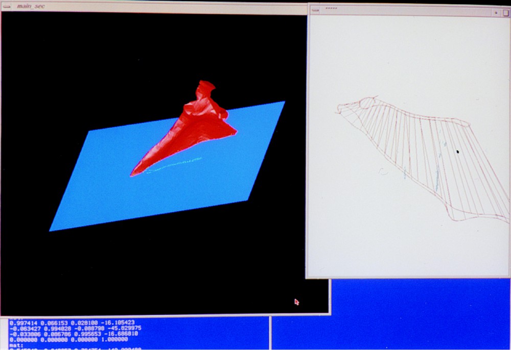
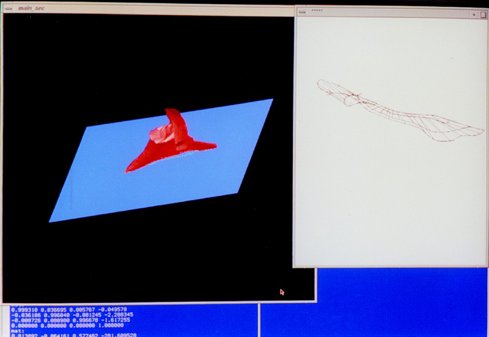
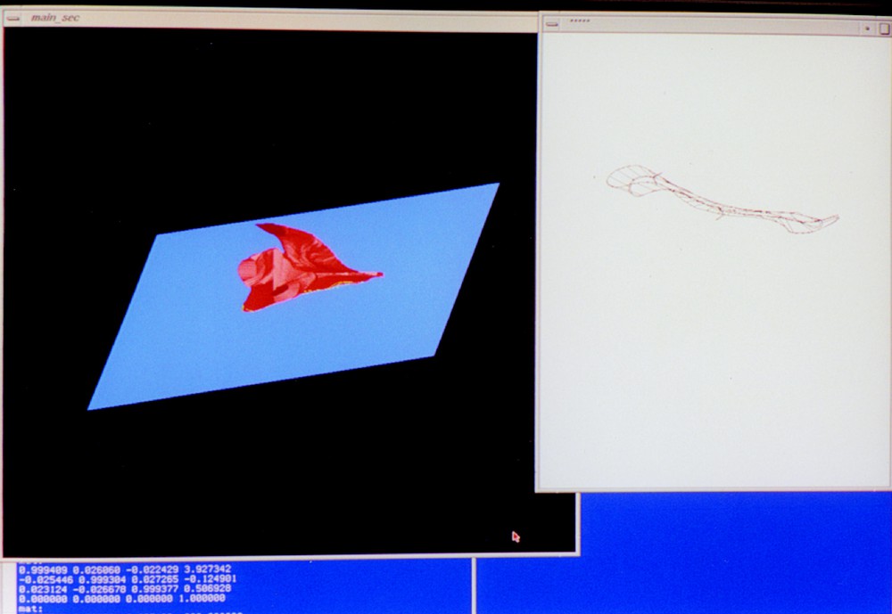
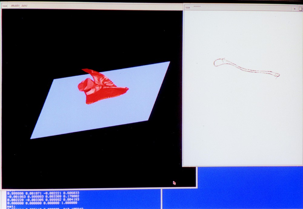
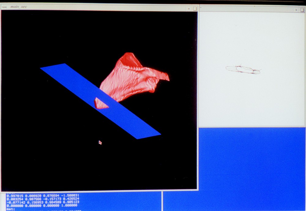
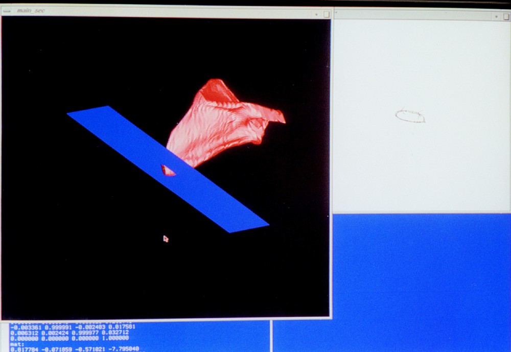
Photographs of the display that monitors the surface and its intersection during their evolution under the algorithm. In the left window, a 3-dimensional scene of the scapula model (red, with the tube hardly visible on it) intersecting the horizontal plane (blue) in which the target curve is drawn (green) can be interactively rotated for inspection. In the right window, a 2-dimensional plot of the two curves to be matched and the discrete mapping cylinder between them. A: starting position and best mapping cylinder (before registration) to a member of the atlas. B, C: two later steps during the same run, D: convergence. E, F: Two steps of an evolution towards a different target curve.
5 Conclusion
The present work shows the feasibility of some registration of a single cross-section to the surface it comes from, using only boundary information. The differential approach is tractable and the generic section algorithm performs well. Many variants and improvements of the present implementation can now be studied. Some theoretical issues such as the existence of valid sectional atlases and the structure of minimal sectional atlases have been raised and formalisms to reformulate and address them have been discussed.
Acknowledgements
Part of this work was done in the Diagnostic Radiology Department of the ‘Hôpital Saint-Louis’, Paris, in collaboration with K. Rachid and M. Laval-Jeantet, as part of the ESPRIT B.R.A. Project 9036.
Version abrégée
Nous décrivons un algorithme permettant, étant donné une surface, un plan et une courbe obtenue par intersection du plan avec cette surface, de retrouver une position de la surface faisant coïncider avec la courbe son intersection avec le plan. Ce problème se pose en imagerie médicale lorsqu'on veut fusionner une image sectionnelle avec des données volumiques déjà acquises dans une autre modalité, comme au cours de la biopsie sous échographie d'une masse après étude tomodensitométrique. L'acquisition des données profite donc ici d'un modèle anatomique préexistant.
L'algorithme est détaillé pour des surfaces polyédrales triangulées et comporte deux parties. La deuxième partie, ou phase locale, finale, consiste en la recherche itérative d'une position adéquate à partir d'une position suffisamment proche d'une solution. Une courbe d'intersection cible est donnée, correspondant à une position inconnue de la surface. À chaque étape, la surface est dans une certaine position, pour laquelle on calcule sa courbe d'intersection, que l'on compare à la courbe cible pour calculer une petite transformation de la surface qui rapproche l'intersection actuelle de la courbe cible. On montre tout d'abord comment, étant donné un champ de déplacement le long d'une courbe d'intersection, il est possible de trouver un déplacement rigide de la surface dont l'effet sur la courbe d'intersection avec le plan approche au mieux le champ de déplacements spécifié. Une technique de moindres carrés est utilisée pour obtenir, en la position actuelle de la surface, un vecteur tangent à l'espace des déplacements rigides dans et dont l'effet approche le champ de déplacement requis. Ce vecteur tangent est un élément de l'algèbre de Lie du groupe des déplacements ; on calcule un vrai déplacement qui l'approche à l'aide d'une formule exacte connue pour l'exponentielle de ce classique groupe de Lie. Le champ de déplacement à approcher le long de la courbe d'intersection est calculé après un appariement, fondé sur les courbures, entre l'intersection actuelle et la cible : il est choisi proportionnel, en chaque sommet du polygone d'intersection, au segment joignant ce sommet au point correspondant de la courbe cible.
La première partie de l'algorithme, ou phase globale, initiale, consiste à trouver une position de départ suffisamment proche d'une solution pour assurer le succès de la phase de recherche locale. À cette fin, on construit pour la surface un atlas sectionnel consistant en un tableau de couples (position de la surface, courbe d'intersection correspondante avec le plan fixe). Une recherche de l'indice donnant le meilleur appariement permet de trouver une meilleure position de départ. L'atlas sectionnel est dit valide si cette procédure mène à une solution quelle que soit la position de départ et la courbe cible. Une condition suffisante de validité est discutée brièvement, ainsi que l'intérêt pour une étude plus approfondie du problème de l'existence d'atlas valides de méthodes de généricité. L'évolution de la position de la surface sous l'influence de l'algorithme est celle de l'état d'un système dynamique, mais ce système dépend de la courbe cible, situation semblable à celle de la Théorie des catastrophes, pour laquelle des hypothèses de généricité apportent de nombreux résultats.
La recherche d'atlas valides minimaux devrait présenter un intérêt, non seulement pour diminuer la complexité des calculs, mais aussi pour comprendre les relations entre la structure du système dynamique sur la position et les caractéristiques géométriques de la surface. L'algorithme programmé est expérimenté sur un modèle d'omoplate reconstruit à partir de données tomodensitométriques.