Bifurcations in a white-blood-cell production model

Samuel Bernard; Jacques Bélair; Michael C. Mackey

doi:10.1016/j.crvi.2003.05.005

Biological modelling / Biomodélisation

Bifurcations in a white-blood-cell production model
[Bifurcations dans un modèle de production de globules blancs]

Présenté par : Pierre Auger

Samuel Bernard ^1,² ; Jacques Bélair ^1,² ; Michael C. Mackey ³

¹ Département de mathématiques et de statistique & Centre de recherches mathématiques, université de Montréal, Montréal, Québec H3C 3J7, Canada
² Centre for Nonlinear Dynamics, McGill University, Montréal, Québec H3G 1Y6, Canada
³ Department of Physiology, Centre for Nonlinear Dynamics, McGill University, 3655 Drummond, Montréal, Québec H3G 1Y6, Canada

Comptes Rendus. Biologies, Volume 327 (2004) no. 3, pp. 201-210.

Résumés

Anglais
Français

We study the dynamics of a model of white-blood-cell (WBC) production. The model consists of two compartmental differential equations with two discrete delays. We show that from normal to pathological parameter values, the system undergoes supercritical Hopf bifurcations and saddle-node bifurcations of limit cycles. We characterize the steady states of the system and perform a bifurcation analysis. Our results indicate that an increase in apoptosis rate of either hematopoietic stem cells or WBC precursors induces a Hopf bifurcation and an oscillatory regime takes place. These oscillations are seen in some hematological diseases.

On étudie la dynamique d'un modèle de production de globules blancs (GB). Le modèle, de nature compartimentale, prend la forme de deux équations différentielles avec deux délais discrets. On montre que la transition de valeurs normales de paramètres à des valeurs pathologiques mène à des bifurcations de Hopf surcritiques ainsi que des bifurcations col–nœud de cycles limites. On caractérise les points fixes du système et on procède à l'analyse des bifurcations. Nos résultats indiquent qu'une augmentation du taux d'apoptose, soit des cellules hématopoı̈étiques, soit des précurseurs des GB, induit une bifurcation de Hopf et qu'un régime oscillatoire apparaı̂t. Ces oscillations sont observées dans certains désordres hématologiques.

Métadonnées

Reçu le : 2003-04-15
Accepté le : 2003-05-23
Publié le : 2004-03-01

PMID

DOI : 10.1016/j.crvi.2003.05.005

Keywords: haematopoiesis, saddle-node and Hopf bifurcation, delay differential equations, oscillation in blood cell, cyclical neutropenia
Mot clés : hématopoı̈èse, bifurcation de Hopf et col-nœud, équations différentielles à retard, oscillation des cellules sanguines, neutropénie cyclique

Affiliations des auteurs :

Samuel Bernard ^{1, 2} ; Jacques Bélair ^{1, 2} ; Michael C. Mackey ³

@article{CRBIOL_2004__327_3_201_0,
     author = {Samuel Bernard and Jacques B\'elair and Michael C. Mackey},
     title = {Bifurcations in a white-blood-cell production model},
     journal = {Comptes Rendus. Biologies},
     pages = {201--210},
     publisher = {Elsevier},
     volume = {327},
     number = {3},
     year = {2004},
     doi = {10.1016/j.crvi.2003.05.005},
     language = {en},
}

TY  - JOUR
AU  - Samuel Bernard
AU  - Jacques Bélair
AU  - Michael C. Mackey
TI  - Bifurcations in a white-blood-cell production model
JO  - Comptes Rendus. Biologies
PY  - 2004
SP  - 201
EP  - 210
VL  - 327
IS  - 3
PB  - Elsevier
DO  - 10.1016/j.crvi.2003.05.005
LA  - en
ID  - CRBIOL_2004__327_3_201_0
ER  -

%0 Journal Article
%A Samuel Bernard
%A Jacques Bélair
%A Michael C. Mackey
%T Bifurcations in a white-blood-cell production model
%J Comptes Rendus. Biologies
%D 2004
%P 201-210
%V 327
%N 3
%I Elsevier
%R 10.1016/j.crvi.2003.05.005
%G en
%F CRBIOL_2004__327_3_201_0

Samuel Bernard; Jacques Bélair; Michael C. Mackey. Bifurcations in a white-blood-cell production model. Comptes Rendus. Biologies, Volume 327 (2004) no. 3, pp. 201-210. doi : 10.1016/j.crvi.2003.05.005. https://comptes-rendus.academie-sciences.fr/biologies/articles/10.1016/j.crvi.2003.05.005/

Version originale du texte intégral

1 Introduction

Hematopoiesis is the term used to describe the production of blood cells. All blood cells come from a unique source, the hematopoietic stem cells (HSC), but mechanisms regulating this production are not completely understood. Particularly, the regulation of leucopoiesis (production of white blood cells) is not well understood and the local HSC regulation mechanisms are even less clear [1–8]. Because of their dynamical character, cyclical neutropenia and other periodic hematological disorders offer us opportunities to better comprehend the nature of these regulatory processes [9].

Cyclical neutropenia (CN) is a rare hematological disorder characterized by oscillations in the circulating white blood cell (WBC) count. Levels of neutrophils, a type of white blood cell, fall from normal to barely detectable levels with a period of 19 to 21 days in humans [4,10,11] and around 14 days in gray collies [4]. These oscillations in the WBC count about a subnormal level are generally accompanied by oscillations around normal levels in other blood cell lineages such as platelets, lymphocytes and reticulocytes [4,7].

The goal of this paper is to study a simple model of WBC production. We look for mechanisms leading to oscillations in the WBC count and relate these mechanisms to physiological features of the hematopoietic system. We use cyclical neutropenia data from a canine model, the gray collie, which is born with this hematological disorder [12].

The paper is organized as follow. In Section 2, we present the model, which is a simple two-compartment production system. In Section 3, we analyze the model using a combination of analytical and numerical continuation methods. It is shown that the positive steady state can be destabilized by a supercritical Hopf bifurcation and that saddle-node bifurcations of limit cycles exist. In Section 4, we discuss the implications for the physiological system of such instabilities.

2 Model

Fig. 1 illustrates the two cell types of this model represented in the two compartments outlined in bold: the hematopoietic stem cells (HSC) and the maturing WBCs. The HSCs are self-renewing and pluripotential (can differentiate into any blood cell type), and the rate at which they differentiate into the WBC line is assumed to be determined by the level of circulating WBCs. As these WBC precursors differentiate, their numbers are amplified by successive divisions. After a certain maturation time τ_M, they become mature WBCs and are released into the blood.

Fig. 1
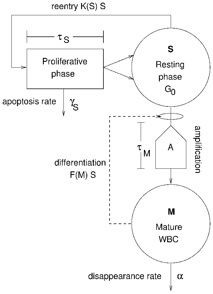
Model of WBC production. The variable S represents the number of hematopoietic stem cells in the resting (G₀) phase. Cells in the resting phase can either enter the proliferative phase at a rate K(S) or differentiate at a rate F(M) to ultimately give rise to mature WBCs M, the second variable. Cells in the HSC proliferative phase undergo apoptosis at a rate γ_S and the cell cycle duration is τ_S. Cells in the differentiation pathway are amplified by successive divisions by a factor, A, which is also used to account for cell loss due to apoptosis. After a time τ_M, differentiated cells become mature WBCs M and are released into the blood. It is assumed that mature WBCs die at a fixed rate α. Two feedback loops control the entire process through the proliferation rate K(S) and the differentiation rate F(M).

As shown in Fig. 1, there are two feedback loops. The first loop is between the mature WBC compartment and the rate F(M) of HSC differentiation into the WBC line. F(M) operates with a delay τ_M that accounts for the time required for WBC division and maturation, so the flux of cells from the resting phase of the HSC compartment is S_{τ_M}F(M_{τ_M}). Here, as elsewhere, the notation x_τ means x(t−τ).

The second feedback loop regulates the rate K(S) at which HSCs re-enter the proliferative cycle from G₀ state, and it operates with a delay τ_S that accounts for the length of time required to produce two daughter HSCs from one mother cell. K(S) is a monotone decreasing function of S and therefore acts as a negative feedback. The flux of cells out of the resting phase of the HSC compartment is given by SK(S). K(S) regulates the level of hematopoietic stem cells (S), while F(M) controls the number of WBCs.

The main agents controlling the peripheral WBC regulatory system through F(M) are the colony stimulating factors (CSFs) such as granulocyte CSF (G-CSF) or granulocyte–monocyte CSF (GM-CSF). The main effect of CSF is stimulating the production of WBCs. As WBCs are a factor in the clearance of CSF, the type of regulation meditated by these cytokines is a negative feedback. An increase of WBC count is followed by a decrease in CSF concentration, leading to a decrease in WBC count, which in turn leads to an increase in CSF concentration, stimulating WBC production.

From Fig. 1 we can write down by inspection the model equations:

\frac{d M}{d t} = - α M + {AS}_{τ_{M}} F (M_{τ_{M}})

(1)

and

\frac{d S}{d t} = - SF (M) - SK (S) + 2 e^{- γ_{S} τ_{S}} S_{τ_{S}} K (S_{τ_{S}})

(2)

The model parameters are the circulating WBC death rate α, the WBC pathway amplification A, the maturation delay of WBC precursors τ_M, the HSC proliferative phase duration τ_S and the apoptotic rate of proliferating HSC, γ_S. The feedback functions F and K are taken as Hill functions:

F (M) = f_{0} \frac{θ_{1}}{θ_{1} + M}

(3)

and

K (S) = k_{0} \frac{θ_{2}^{s}}{θ_{2}^{s} + S^{s}}

(4)

All parameters describe physiological quantities and are de facto assumed to be positive. Table 1 shows the parameter values used in this study. Some of them can be evaluated from experimental data found in the literature, and references are indicated in Table 1. However, the values of parameters such as $S_{*}$ , τ_M and parameters inside the feedback loops are less clear. A recent study [13] indicates that the absolute stem cell population would be conserved in mammals. This implies that the frequency $S_{*}$ would be much lower in dogs (our model) than in mice (where the data come from). Moreover, many parameters depends on $S_{*}$ such as A and τ_M. Nevertheless, numerical simulations have shown that changing the value of $S_{*}$ (along with A and τ_M) does not change the dynamics qualitatively, and not much quantitatively. For these reasons, we will take the steady state stem cell count $S_{*}$ found in mice.

Parameter	Unit	Value	References
A	100	20	[8,17]
f ₀	day⁻¹	0.8	[7]
θ ₁	10⁶ cell kg⁻¹	0.36	model
f ₀	day⁻¹	8.0	model
θ ₂	10⁶ cell kg⁻¹	0.095	model
s		2∼3	[18–20]
τ _M	day	3.5	[14,21,22]
τ _S	day	2.8	[8,23]
γ _S	day⁻¹	0.07	[8]
α	day⁻¹	2.4	[24]
$S_{*}$	10⁶ cell kg⁻¹	1.1	[8,25]
$M_{*}$	10⁶ cell kg⁻¹	6.9	[7,8]
$F_{*}$	day⁻¹	0.04	[8]
$K_{*}$	day⁻¹	0.06	[8]

In normal condition, the duration of WBC transit time from the most primitive precursor cells to fully mature cells has been evaluated to approximately 12 days [14], the post-mitotic maturation phase to about 3.0 days in dogs [7]. Some authors even report a transit time of 42 days or more [15]. However, clinical data show that the transit time is shortened in CN patients or after granulocyte colony stimulating factor (G-CSF) administration. Considering that the hematopoietic regulatory system acts thorough the maturation cell line, we will take the feedback delay τ_M=3.5 days (in a recent study [16], primitive murine blood cells have been shown to divide up to 8 times in a 3-day in vitro culture). Numerical simulations show that large changes in τ_M (up to 42 days) do not affect significantly the behavior of the solution, although the solution may become apparently quasi-periodic in some ranges of τ_M values.

3 Analysis

In this section, we analyze the stability of steady states and their bifurcations. As the parameter space is vast, we have to choose the most relevant parameters to be examined. A key feature in the onset of hematopoietic disorders such as CN and PCML seems to be the apoptosis rate of blood cell precursors. In the present model, two parameters control this apoptotic rate, the HSC apoptosis rate γ_S and the precursor amplification A, which can be expressed as:

A = 2^{q} \exp (- γ_{p} T)

(5)

The parameter A is composed of an absolute amplification term 2^q representing q successive divisions, and of a term representing the surviving fraction from apoptosis, exp(−γ_PT), where γ_P is the precursor apoptosis rate and T the time during which the apoptosis occurs. Therefore, our two main bifurcation parameters are γ_S and A. Other parameters are fixed as in Table 1 unless otherwise noted.

3.1 Linear stability. Quasi-steady-state assumption

In this section, we consider a simpler model by assuming the function F to be constant. This uncouples Eqs. (1) and (2) and allows a complete stability analysis of the stem cell compartment. In that case, it is easy to show that a single positive steady state exists for the system if F<k₀r, where r=2exp(−γ_Sτ_S)−1. The following relation defines the nonzero steady states,

S_{*}^{s} = θ_{2}^{s} [\frac{k_{0} r}{F} - 1]

(6)

When the apoptosis rate is increased to

γ_{S} = \frac{1}{τ_{S}} \ln [\frac{2}{F / k_{0} + 1}]

(7)

the positive steady state reaches, and collapses with, the null steady state. The linearization around the positive steady state of Eq. (2) allows us to understand the nature of this bifurcation. Let

y = S - S_{*}

, so the linearized equation from Eq. (2) is

\dot{y} = - A_{+} y - B_{+} y_{τ_{S}}

(8)

where the parameters A₊ and B₊ are defined by

A_{+} = F + [(1 - s) \frac{F}{r} + s \frac{F^{2}}{k_{0} r^{2}}]

(9)

and

B_{+} = - (r + 1) [(1 - s) \frac{F}{r} + s \frac{F^{2}}{k_{0} r^{2}}]

(10)

The characteristic equation associated with Eq. (8) is:

λ + A_{+} + B_{+} \exp (- λ τ_{S}) = 0

(11)

Let us recall a well-known theorem [26,27] on linear-delay differential equations. The steady state leading to the characteristic equation (11) is locally stable if and only if:

| B_{+} | < A_{+}

(12)

B_{+} > | A_{+} | and τ_{S} < \frac{\arccos (- A_{+} / B_{+})}{\sqrt{B_{+}^{2} - A_{+}^{2}}}

(13)

When F=k₀r, the only steady state is zero. If the apoptosis rate γ_S is decreased by a small amount, we can assume that, for small ε>0,

\frac{F}{k_{0} r} = 1 - ϵ

(14)

In that case, we can show that

| B_{+} | = \frac{F}{r} (1 - s ϵ) + F (1 - s ϵ) < \frac{F}{r} (1 - s ϵ) + F = A_{+}

(15)

and thus the positive steady state is locally stable when it is close to zero.

Now, if we linearize around the trivial steady state, we find a linearized equation (with z=S)

\dot{z} = - A_{0} z - B_{0} z_{τ_{S}}

(16)

with

A_{0} = F + k_{0} and B_{0} = - (r + 1) k_{0}

(17)

Two cases have to be considered. First, if F⩾k₀r, then

A_{0} ⩾ k_{0} r + k_{0} = | B_{0} |

(18)

implying that the null steady state is stable. In the other case, F<k₀r, then

A_{0} < k_{0} r + k_{0} = - B_{0}

(19)

and the trivial steady state is unstable.

We have thus shown that when γ_S takes the value given by Eq. (7), the unique positive steady state collapses with the trivial steady state, leading to a bifurcation point. In order to distinguish between the different possible bifurcations, we have to look at the value of the exponent s in the feedback function K. If s is even, then the s-root in Eq. (6) is not real when F>k₀r, so only the trivial steady state exists. When γ_S decreases, leading to an increase of r, a pair of nonzero steady states appears around zero, giving a pitchfork bifurcation. If s is odd, then the s-root always exists. When γ_S decreases, the steady state $S_{*}$ goes from negative to positive, and there is an exchange of stability at zero: this is a transcritical bifurcation.

3.1.1 Oscillation around the positive steady state

There exists a range of γ_S for which the positive steady state $S_{*}$ is unstable. Fig. 2 shows the bifurcation diagram of S with respect to γ_S.

Fig. 2
Left panel: bifurcation diagram with apoptosis rate γ_S as a parameter. The positive steady state is represented by the thin line and the envelope of the periodic solution by the thick line. The other parameter values are F=0.05, θ₁=1.0, k₀=1.77, τ_S=2.2 and s=3. In this case, a transcritical bifurcation occurs at point II. At point O, a supercritical Hopf bifurcation occurs and a stable limit cycle appears. This limit cycle eventually disappears through a reverse supercritical Hopf bifurcation at point I. Right panel: profiles of periodic solutions for values of γ_S between 0.24 and 0.28 (points O and I in the right panel). The periodic solutions have been rescaled on a time t′ so that each solution has a period T=1. For a given value of γ_S, the vertical axis is the HSC count as a function of t′ over one period.

Many authors have speculated about the consequences of such oscillations. There might be a causal link between oscillation in the HSC compartment and oscillations seen in hematological disorders such as periodic chronic myelogenous leukemia or cyclical neutropenia.

3.2 Analysis of the full model

In this section, we focus on the behavior of the solution of the full model as the parameter A is varied. It is shown that a supercritical Hopf bifurcation destabilizes the positive fixed point and that for an interval of values of A, there is bistability. When A approaches 0, the steady state value $M_{*}$ approaches 0, while $S_{*}$ stays positive, and a limit cycle coexists with the steady state.

3.2.1 Existence and uniqueness of the positive steady state

The full model described by Eqs. (1) and (2) cannot be easily analyzed. However, by restricting the parameter space, we can give a condition for a single positive steady state to exist. In particular, we take:

f_{0} < (1 - \frac{1}{s}) {rk}_{0} = (1 - \frac{1}{s}) (2 \exp (- γ_{S} τ_{S}) - 1) k_{0}

(20)

and show that there exists a single positive steady state for Eqs. (1), (2), denoted

(M_{*}, S_{*})

through the rest of the paper. In this section, we present a proof for the existence and uniqueness of the positive steady state under condition (20). First write the equation for the steady state of M. From Eq. (1) we have

M_{*}

defined by:

α M_{*} = {AS}_{*} F (M_{*})

(21)

From Eq. (21) and the steady state equation for

S_{*}

, (6), we can eliminate

S_{*}

, and obtain:

M_{*} = \frac{A θ_{2}}{α} \sqrt[s]{(\frac{{rk}_{0}}{F (M_{*})} - 1)} F (M_{*})

(22)

Let the right-hand side of Eq. (22) be denoted $G (M_{*})$ . Then the derivative of G with respect to $M_{*}$ is:

G' (M_{*}) = \frac{A θ_{2}}{s α} \sqrt[s]{(\frac{{rk}_{0}}{F (M_{*})} - 1)} F' (M_{*}) [s - \frac{1}{1 - F (M_{*}) {({rk}_{0})}^{- 1}}]

(23)

If we can prove that $G' (M_{*})$ is always negative, then by using the fixed-point theorem, it is easy to show that there exists a unique positive steady state $M_{*}$ , and from that value the uniqueness of the steady state $S_{*}$ follows naturally. To show that $G' (M_{*})$ is negative, we must verify that the factor in the brackets in Eq. (23) is positive since the others factors are negative (from the definition of F(M) in Eq. (3), it is obvious that F′(M)<0). So we need to find conditions for which:

s - \frac{1}{1 - F (M_{*}) {({rk}_{0})}^{- 1}} > 0

(24)

which is equivalent to showing that

F (M_{*}) < (1 - \frac{1}{s}) {rk}_{0}

(25)

We know that

F (M_{*}) < f_{0}

, so a sufficient condition for

G' (M_{*})

to be negative is:

f_{0} < (1 - \frac{1}{s}) {rk}_{0} = (1 - \frac{1}{s}) (2 \exp (- γ_{S} τ_{S}) - 1) k_{0}

(26)

which completes the proof of the existence and uniqueness of the steady state

(M_{*}, S_{*})

under condition (20).

3.2.2 Characteristic equation of the model

The linearization of Eqs. (1) and (2) around the unique positive steady state $(M_{*}, S_{*})$ is performed along the same lines as above. First define new variables $x = M - M_{*}$ and $y = S - S_{*}$ so that x=0 and y=0 are the coordinates of the fixed point. Then by linearizing around the steady state $(M_{*}, S_{*})$ , we obtain:

\frac{d x}{d t} = A_{1} x + A_{2} x_{τ_{M}} + A_{3} x_{τ_{M}}

(27)

and

\frac{d y}{d t} = B_{1} x + B_{2} y + B_{3} y_{τ_{S}},

(28)

where the linearization coefficients are: (29)

The subscripts in the equalities denote the partial derivative with respect to the variable and the star subscript $(*)$ means that the function is evaluated at the steady state. The prime stands for the derivative with respect to the argument. These equations can be formulated in vector form,

\frac{d X}{d t} = LX + R_{M} X_{τ_{M}} + R_{S} X_{τ_{S}}

(30)

where

X = (\begin{matrix} x \\ y \end{matrix}), L = (\begin{matrix} A_{1} & 0 \\ B_{1} & B_{2} \end{matrix})

R_{M} = (\begin{matrix} A_{2} & A_{3} \\ 0 & 0 \end{matrix}), R_{S} = (\begin{matrix} 0 & 0 \\ 0 & B_{3} \end{matrix})

The characteristic equation of Section 3.2.2 is defined as:

\det [λ I - L - R_{M} \exp (- λ τ_{M}) - R_{S} \exp (- λ τ_{S})] = 0

(31)

with I the 2×2 identity matrix. The characteristic equation can then be explicitly written:

λ^{2} - (A_{1} + B_{2}) λ - A_{2} λ e^{- λ τ_{M}} - B_{3} λ e^{- λ τ_{S}} + B_{2} A_{1} + (A_{2} B_{2} + B_{1} A_{3}) e^{- λ τ_{M}} + A_{1} B_{3} e^{- λ τ_{S}} + A_{2} B_{3} e^{- λ (τ_{M} + τ_{S})} = 0

(32)

The locations of the roots of Eq. (32) will give information about the local stability of the steady state $(M_{*}, S_{*})$ . In Section 3.2.3, numerical methods are used to study the location of the roots of Eq. (32).

3.2.3 Bifurcation analysis of the full model

The condition defined by Eq. (20) restricts the values taken by γ_S. Indeed, from Eq. (20), we find:

γ_{S} < \frac{1}{τ_{S}} \ln [\frac{2 (s - 1) k_{0}}{{sf}_{0} + (s - 1) k_{0}}]

(33)

The right-hand side of this inequality is slightly smaller than the right-hand side of Eq. (7). Moreover, numerical simulations when γ_S approaches this value show that the behavior of the solution is highly irregular. Therefore, we concentrate our analysis on the behavior of solutions as the amplification parameter A is varied and keep γ_S well below the critical value defined by Eq. (33).

The fixed-point equations are defined by setting the left-hand sides of Eqs. (1), (2) equal to zero. Solving for the nonzero steady states leads to

M_{*} = \frac{A}{α} S_{*} F (M_{*})

(34)

and

S_{*}^{s} = θ_{2}^{s} [\frac{k_{0} r}{F (M)} - 1]

(35)

Eq. (34) can be expressed as a 2s-th order polynomial in

M_{*}

by replacing

S_{*}

by its steady-state value. Generally,

{(M_{*}^{2} + θ_{1} M_{*})}^{s} = {(\frac{A}{α} f_{0} θ_{1} θ_{2})}^{s} (\frac{k_{0} r}{f_{0} θ_{1}} (θ_{1} + M_{*}) - 1)

(36)

In the particular case where s=2, the steady-state equation becomes a fourth-order polynomial:

α^{2} M_{*}^{4} + 2 α^{2} θ_{1} M_{*}^{3} + α^{2} θ_{1}^{2} M_{*}^{2} - A^{2} f_{0} θ_{1} θ_{2}^{2} {rk}_{0} M_{*} - A^{2} f_{0}^{2} θ_{1}^{2} θ_{2}^{2} (\frac{{rk}_{0}}{f_{0}} - 1) = 0

(37)

This equation can be solved analytically using symbolic computation software such as Maple. At A=0, Eq. (37) simplifies and it is easy to show that there exists a double zero root and a double negative root. For A>0, as shown above, only one root is positive. With parameter values as in Table 1 and A=0, the system (1), (2) is unstable, since the characteristic equation (32) reduces to Eq. (11) and the values of the coefficients are A₊=−0.056 and B₊=1.41. As B₊>|A₊|, the condition for stability of the nonzero steady state when A=0 is then, from condition (13), τ_S<1.09. This condition is not satisfied, since τ_S takes larger values. When 0<A⪡1, by continuity, the stability of system (1), (2) does not change. At A=0, there is an unstable steady state $(M_{*} \equiv 0, S_{*} > 0)$ accompanied by a stable limit cycle in the S variable only and of zero amplitude in M. When A is increased, the unstable steady state becomes positive $(M_{*} > 0, S_{*} > 0)$ and the amplitude of the limit cycle becomes nonzero in both M and S. As A is further increased, the analysis becomes much more difficult and the bifurcation study cannot be carried out with symbolic tools only.

At this point, one must use numerical methods in order to understand the complexity of the system. To perform the numerical analysis, we used a Matlab package, DDE-BIFTOOLS [28], which is based on continuation methods that are in widespread use for ordinary differential equations through the software AUTO [29]. This package is well suited for analysis of delay differential equations.

In Fig. 3 we show bifurcation diagrams of M and S as well as their periodic solution profiles. If we follow the evolution of the steady state $(M_{*}, S_{*})$ as the parameter A is decreased, a supercritical Hopf bifurcation occurs (points O in Fig. 3, left panels). At this point, a small-amplitude stable limit cycle appears, and disappears in a saddle-node bifurcation (points I) together with an unstable limit cycle. This unstable limit cycle had appeared previously in another saddle-node bifurcation (points II), with a large amplitude stable limit cycle. The large amplitude limit cycle exists from point II to A=0. In the right panels of Fig. 3, the limit cycle profiles are shown. The time axis in right panels of Fig. 3 are rescaled so that the period T=1. It should be noted that when the amplification A ranges in typical CN values (10 to 30), the period of oscillation is between 13 and 17 days, which is in the average for CN in gray collies.

Fig. 3
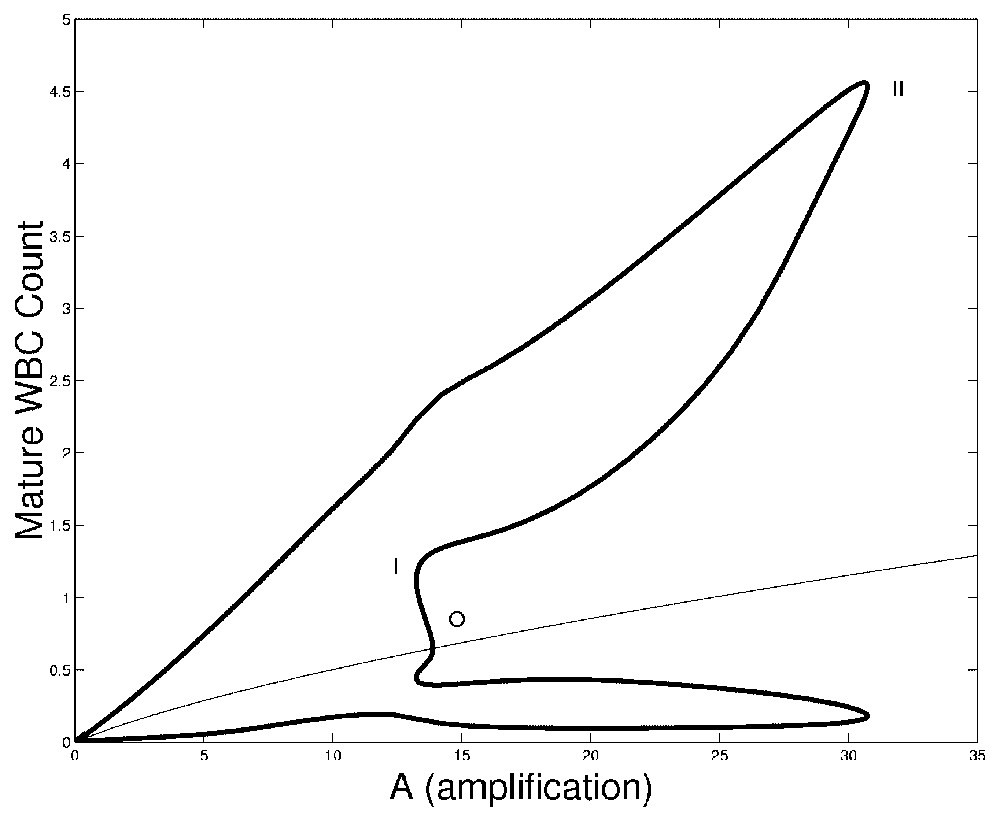
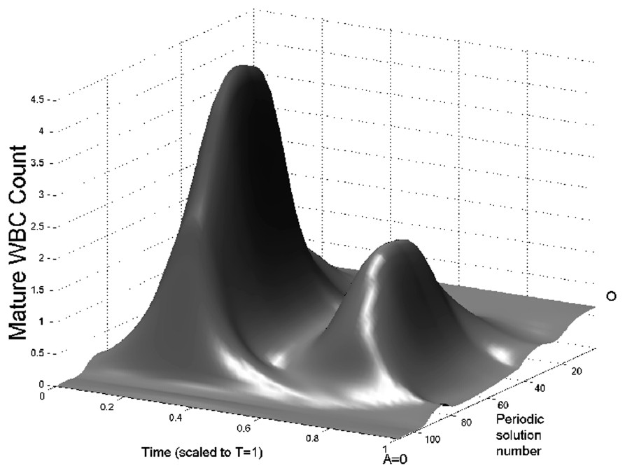
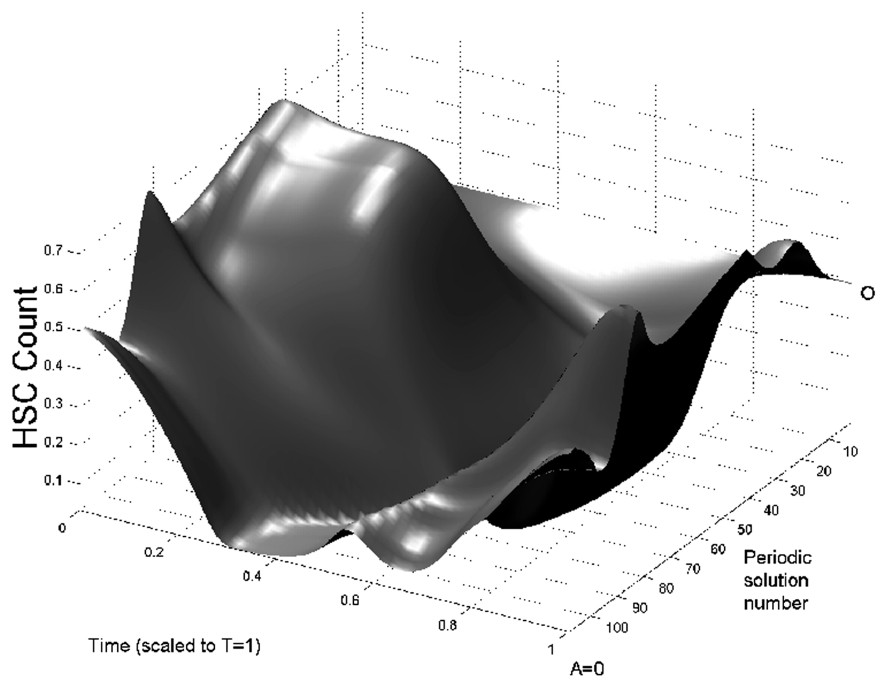
Bifurcation diagram of the full model (Eqs. (1) and (2)) as a function of A. On left panels, the bifurcation diagrams of mature WBC $M_{*}$ (upper panel) and HSC $S_{*}$ (lower panel) are shown. In each panel the thin line is the corresponding steady state and the thick lines are the envelopes of periodic solutions. Between points O and I is a small amplitude stable periodic solution. Between points I and II, there is an unstable period solution and from point II to A=0, there is a large amplitude stable periodic solution. Right panels: surface representation of periodic solutions when the amplification A is varied. The periodic solutions in M are represented in upper right panel and the periodic solutions in S are represented in lower right panel. Periodic solution number 0 corresponds to points O in left panels, and numbers 108 to A=0. To plot this surface, the bifurcation curves in left panels have been ‘unfolded’, so there is only one periodic solution represented at a time. See the caption of Fig. 2 for more details.

4 Discussion

We have analyzed a simple model of white-blood-cell production. Oscillations in blood-cell count have been observed in many hematological diseases such as cyclical neutropenia (CN) or periodic myelogenous leukemia (PCML) [30]. In both diseases, an alteration in the apoptotic rate of white-blood-cell precursors has been observed. The goal of the present paper was to establish, using a simple model, if these changes in apoptosis rates could explain the onset of oscillations. It has been shown in Section 3 that the elevation of the apoptosis rate is a sufficient condition for the onset of oscillations in the WBC count. This elevation has been observed in neutrophil precursors in CN patients. We make the hypothesis that this elevation in neutrophil precursor apoptosis rate is the cause of oscillation seen in CN.

The case of PCML is less clear. This form of leukemia is characterized by oscillations from normal to high levels of WBC with periods ranging from 35 to 80 days. A relationship exists between CN and certain forms of leukemia, since some CN patients eventually develop these leukemias [31–35]. However, experimental data show that leukemic cells have a decreased rate of apoptosis. The model presented here does not display any oscillatory behavior when apoptosis rate is decreased below normal. Further investigations will have to be carried out to establish a link between dynamics seen in CN and PCML.

Acknowledgements

MCM is supported by the Natural Sciences and Engineering Research Council (NSERC Grant No. OGP-0036920, Canada), MITACS (Canada), and the ‘Fonds pour la formation de chercheurs et l'aide à la recherche’ (FCAR Grant No. 98ER1057, Québec, Canada), and the Leverhulme Trust (UK). JB is supported by the Natural Sciences and Engineering Research Council (NSERC Grant No. OGP-0008806, Canada), MITACS (Canada), and the ‘Fonds pour la formation de chercheurs et l'aide à la recherche’ (FCAR Grant No. 98ER1057, Québec, Canada). SB is supported by MITACS (Canada) and the ‘Institut des sciences mathématiques’ (ISM, Québec, Canada).

Bibliographie

[1] S.I. Rubinow; J.L. Lebowitz A mathematical model of neutrophil production and control in normal man, J. Math. Biol., Volume 1 (1975), pp. 187-225

[2] N. MacDonald Cyclical neutropenia: models with two cell types and two time lags (A. Valleron; P. Macdonald, eds.), Biomathematics and Cell Kinetics, Elsevier/North-Holland, Amsterdam, 1978, pp. 287-295

[3] T. Hearn; C. Haurie; M.C. Mackey Cyclical neutropenia and the peripheral control of white-blood-cell production, J. Theor. Biol., Volume 192 (1998), pp. 167-181

[4] C. Haurie; D.C. Dale; M.C. Mackey Cyclical neutropenia and other periodic haematological diseases: a review of mechanisms and mathematical models, Blood, Volume 92 (1998), pp. 2629-2640

[5] C. Haurie; D.C. Dale; M.C. Mackey Occurrence of periodic oscillations in the differential blood counts of congenital, idiopathic and cyclical neutropenic patients before and during treatment with G-CSF, Exp. Hematol., Volume 27 (1999), pp. 401-409

[6] C. Haurie; R. Person; D.C. Dale; M.C. Mackey Haematopoietic dynamics in grey collies, Exp. Hematol., Volume 27 (1999), pp. 1139-1148

[7] C. Haurie; D.C. Dale; R. Rudnicki; M.C. Mackey Modeling complex neutrophil dynamics in the grey collie, J. Theor. Biol., Volume 204 (2000), pp. 505-519

[8] M.C. Mackey Cell kinetic status of hematopoietic stem cells, Cell Prolif., Volume 34 (2001), pp. 71-83

[9] G.K. von Schulthess; N.A. Mazer Cyclic neutropenia (CN): a clue to the control of granulopoiesis, Blood, Volume 59 (1982), pp. 27-37

[10] D. Guerry; D.C. Dale; M. Omine; S. Perry; S.M. Wolff Periodic hematopoiesis in human cyclic neutropenia, J. Clin. Investig., Volume 52 (1973), pp. 3220-3230

[11] D.C. Dale; W.P. Hammond Cyclic neutropenia: a clinical review, Blood Rev., Volume 2 (1988), pp. 178-185

[12] J.E. Lund; G.A. Padgett; R.L. Ott Cyclic neutropenia in grey collie dogs, Blood, Volume 29 (1967), pp. 452-461

[13] J.L. Abkowitz; S.N. Catlin; M.T. McCallie; P. Guttorp Evidence that the number of hematopoietic stem cells per animal is conserved in mammals, Blood, Volume 100 (2002), pp. 2665-2667

[14] J.L. Lebowitz; S.I. Rubinow Grain count distributions in labeled cell populations, J. Theor. Biol., Volume 23 (1969), pp. 99-123

[15] I. Østby; L.S. Rusten; G. Kvalheim; P. Grøttum A mathematical model for reconstitution of granulopoiesis after high-dose chemotherapy with autologous stem cell transplantation, J. Math. Biol., Volume 47 (2003), pp. 101-136

[16] R.A. Oostendorp; J. Audet; C.J. Eaves High-resolution tracking of cell division suggests similar cell cycle kinetics of haematopoietic stem cells stimulated in vitro and in vivo, Blood, Volume 95 (2000), pp. 855-862

[17] J.P. Novak; E. Nečas Proliferation differentiation pathways of murine haematopoiesis: Correlation of lineage fluxes, Cell Prolif., Volume 27 (1994), pp. 597-633

[18] L.K. Andersen; M.C. Mackey Resonance in periodic chemotheray: a case study of acute myelogenous leukemia, J. Theor. Biol., Volume 209 (2001), pp. 113-130

[19] L. Niu; D.W. Golde; J.C. Vera; M.L. Heaney Kinetic resolution of two mechanisms for high-affinity granulocyte–macrophage colony-stimulating factor binding to its receptor, Blood, Volume 94 (1999), pp. 3748-3753

[20] C.J. Bagley; J.M. Woodcock; F.C. Stomski; A.F. Lopez The structural and functional basis of cytokine receptor activation: lessons from the common subunit of the granulocyte–macrophage colony-stimulating factor, interleukin-3 (IL-3), and IL-5 receptors, Blood, Volume 89 (1997), pp. 1471-1482

[21] M. Nakamura, Estimation of cell cycle parameters from cell division tracking data, Master's thesis, University of New South Wales, 1999

[22] J. Burthem, R. Mottram, G.S. Lucas, A.D. Whetton, Imatinib mesilate (STI571) causes an increased rate of maturation and a reduced expansion of cell number during the granulocytic differentiation of CD34+ cells from CML patients, unpublished

[23] S. Cheshier; S. Morrison; X. Liao; I. Weissman In vivo proliferation and cell cycle kinetics of long term self renewing haematopoietic stem cells, Proc. Natl Acad. Sci. USA, Volume 96 (1999), pp. 3120-3125

[24] K.A. Deubelbeiss; J.T. Dancey; L.A. Harker; C.A. Finch Neutrophil kinetics in the dog, J. Clin. Investig., Volume 55 (1975), pp. 833-839

[25] L. Edelstein-Keshet; A. Israel; P. Lansdorp Modelling perspective on aging: can mathematics help us stay young?, J. Theor. Biol., Volume 213 (2001), pp. 509-525

[26] N. Hayes Roots of the transcendental equation associated with a certain difference-differential equation, J. Lond. Math. Soc., Volume 25 (1950), pp. 226-232

[27] S. Bernard; J. Bélair; M.C. Mackey Sufficient conditions for stability of linear differential equations with distributed delay, Discrete Contin. Dyn. Syst. Ser. B, Volume 1 (2001), pp. 233-256

[28] K. Engelborghs, T. Luzyanina, G. Samaey, DDE-BIFTOOL v. 2.00: a Matlab package for bifurcation analysis of delay differential equations, Katholieke Universiteit Leuven, 2001, http://www.cs.kuleuven.ac.be/koen/

[29] E.J. Doedel Auto: a program for the automatic bifurcation analysis of autonomous systems, Proc. 10th Manitoba Conf. on Num. Math. Comput., University of Manitoba, Winnipeg, Canada, 1981, pp. 265-284

[30] P. Fortin; M.C. Mackey Periodic chronic myelogenous leukemia: spectral analysis of blood cell counts and aetiological implications, Brit. J. Haematol., Volume 104 (1999), pp. 336-345

[31] D.B. Lensink; A.B. Barton; R.R. Appelbaum; W.P. Hammond Cyclic neutropenia as a premalignant manifestation of acute lymphoblastic leukemia, Am. J. Hematol., Volume 22 (1986), pp. 9-16

[32] M.E. Weinblatt; P. Scimeca; A. James-Herry; I. Sahdev; J. Kochen Transformation of congenital neutropenia into monosomy 7 and acute nonlymphoblastic leukemia in a child treated with granulocyte colony-stimulating factor, J. Pediatr., Volume 126 (1995), pp. 263-265

[33] M.H. Freedman; M.A. Bonilla; C. Fier; A.A. Bolyard; D. Scarlata; L.A. Boxer; S. Brown; B. Cham; G. Kannourakis; S.E. Kinsey; P.G. Mori; T. Cottle; K. Welte; D.C. Dale Myelodysplasia syndrome and acute myeloid leukemia in patients with congenital neutropenia receiving G-CSF therapy, Blood, Volume 96 (2000), pp. 429-436

[34] S. Jeha; K.W. Chan; A.G. Aprikyan; W.K. Hoots; S. Culbert; H. Zietz; D.C. Dale; M. Albitar Spontaneous remission of granulocyte colony-stimulating factor-associated leukemia in a child with severe congenital neutropenia, Blood, Volume 96 (2000), pp. 3647-3649

[35] M.C. Dinauer; J.A. Lekstrom-Himes; D.C. Dale Inherited neutrophil disorders: molecular basis and new therapies, Hematology, Volume 2000 (2000), pp. 303-318

Commentaires - Politique

Ces articles pourraient vous intéresser

Contribution to the study of periodic chronic myelogenous leukemia

Laurent Pujo-Menjouet; Michael C. Mackey

C. R. Biol (2004)

On the stability of hematopoietic model with feedback control

Catherine Marquet; Mostafa Adimy

C. R. Math (2012)

Contribution of a mathematical modelling approach to the understanding of the ovarian function

Frédérique Clément; Danielle Monniaux; Jean-Christophe Thalabard; ...

C. R. Biol (2002)