Plan
Comptes Rendus

Biological modelling / Biomodélisation
Cell cycle progression
Comptes Rendus. Biologies, Volume 327 (2004) no. 3, pp. 193-200.

Résumé

In this paper we consider cell cycle models for which the transition operator for the evolution of birth mass density is a simple, linear dynamical system with a stochastic perturbation. The convolution model for a birth mass distribution is presented. Density functions of birth mass and tail probabilities in n-th generation are calculated by a saddle-point approximation method. With these probabilities, representing the probability of exceeding an acceptable mass value, we have more control over pathological growth. A computer simulation is presented for cell proliferation in the age-dependent cell cycle model. The simulation takes into account the fact that the age-dependent model with a linear growth is a simple linear dynamical system with an additive stochastic perturbation. The simulated data as well as the experimental data (generation times for mouse L) are fitted by the proposed convolution model.

Métadonnées
Reçu le :
Accepté le :
Publié le :
DOI : 10.1016/j.crvi.2003.05.002
Mots clés : cell cycle, mass distribution, convolution, saddle-point approximation, maximum likelihood
Joanna Tyrcha 1

1 Department of Mathematical Statistics, Institute of Mathematics, Stockholm University, S-106 91 Stockholm, Sweden
@article{CRBIOL_2004__327_3_193_0,
     author = {Joanna Tyrcha},
     title = {Cell cycle progression},
     journal = {Comptes Rendus. Biologies},
     pages = {193--200},
     publisher = {Elsevier},
     volume = {327},
     number = {3},
     year = {2004},
     doi = {10.1016/j.crvi.2003.05.002},
     language = {en},
}
TY  - JOUR
AU  - Joanna Tyrcha
TI  - Cell cycle progression
JO  - Comptes Rendus. Biologies
PY  - 2004
SP  - 193
EP  - 200
VL  - 327
IS  - 3
PB  - Elsevier
DO  - 10.1016/j.crvi.2003.05.002
LA  - en
ID  - CRBIOL_2004__327_3_193_0
ER  - 
%0 Journal Article
%A Joanna Tyrcha
%T Cell cycle progression
%J Comptes Rendus. Biologies
%D 2004
%P 193-200
%V 327
%N 3
%I Elsevier
%R 10.1016/j.crvi.2003.05.002
%G en
%F CRBIOL_2004__327_3_193_0
Joanna Tyrcha. Cell cycle progression. Comptes Rendus. Biologies, Volume 327 (2004) no. 3, pp. 193-200. doi : 10.1016/j.crvi.2003.05.002. https://comptes-rendus.academie-sciences.fr/biologies/articles/10.1016/j.crvi.2003.05.002/

Version originale du texte intégral

1 Introduction

The cell cycle is normally defined as the period from cell birth to its division into two daughter cells. The most significant aspect of cell growth is the synthesis of new cellular material, such as proteins, and the initiation of DNA synthesis is one of the first observable cell cycle landmarks. There are cells that are characterized by uncontrolled growth. It is of greatest interest to find answer to the question what causes the cell to begin initiation of DNA synthesis, since this problem is closely connected with explaining the cause of pathological growth, such as in cancer.

Many mathematical models were proposed which explain the asymptotic stability of the cell cycle. By the stability concept we mean the stability of the line: mother–daughter–granddaughter–great-grand-daughter, etc. We derive a recursion relation for the distribution of cell mass at birth in a sample of cells in the generation n given the distribution in the generation n−1. We prove the existence of a unique, asymptotically stable, limiting mass distribution. An alternative convention suggested, among others, by Harris [1] and Jagers [2] is to choose samples from all cells present in the culture at a particular instant of time, and investigate stabilization of the mass distribution in the population as time passes.

The cell cycle is one of many examples of systems that have a mixture of deterministic and probabilistic dynamics. Many other examples may be found in [3]. In this paper we develop a general modelling framework for such systems.

First, we shortly review previous cell cycle models and the mathematical tools used to investigate the asymptotic stability of the mass distribution at birth. We concentrate on the models that represent linear dynamical systems with a stochastic perturbation. In Section 3, we present the convolution model for estimating distributions of cell mass at birth. In Section 4, we describe our simulation procedure. In Section 5, we present the maximum likelihood method for estimate parameters in our convolution model and finally show how the theoretical density functions of cell mass birth fit both our simulated and experimental data.

2 Background

The cell mass at birth (x) may be considered as a random variable. If we denote by f the density function of the mass distribution at birth for a mother cell then Pf denotes the density function of the mass distribution at birth for daughter cells. In general the operator P has the form

Pf (x)=0K(x,y)f(y)dy(1)
where K is to be thought of as the conditional probability that, given a mass y in the previous generation, we will have a mass x in the current generation. K is a stochastic Markov kernel, which means:
0K(x,r)dx=1 for r0 and
K(x,r)0 for x0,r0

The particular form of the kernel K(x,y) depends on the assumptions concerning the mass growth and the probability of division. Depending on these assumptions we can distinguish, among others, the following models of the cell cycle: the mitogen model [4], the tandem model [5], the probabilistic model [6,7], and the generalized mitogen model [8]. In all these models, the authors studied asymptotic properties of the sequence of iterates {Pn} (Pn denotes the mass density function in the n-th generation).

In the paper by Lasota, Mackey and Tyrcha [9], we developed a general modelling framework for the treatment of the statistical dynamics of systems in which easily identifiable events occur at irregular times. The desired recurrence relation between successive mass levels at event occurrence is given by:

xn+1=λ-1Q-1Q(xn)+τn for n=0,1,(2)
where, by assumption, xn and τn are independent stochastic variables. We assume that Q and λ satisfy the following conditions:
  • – the functions Q:R+R+ and λ:R+R+ are non-decreasing and absolutely continuous on each subinterval [0,c] on the half-line R+;
  • Q(0)=λ(0)=0 and lim nQ(x)= lim xλ(x)=.

In interpreting the cell division cycle within the context of the general model presented in [9], we associate the occurrence of an event with a triggering of the process, which ultimately leads to mitosis and cytokinesis.

The class of models proposed by Lasota and Mackey [4], Tyson and Hannsgen [5] and Tyrcha [8] satisfies all of the conditions of the general model described above and in [9]. Furthermore, the quantities of mass in consecutive generations of newly born cells satisfy the recurrence relation (2) with τn having a survival function ex. Setting zn=Q[λ(xn)], the transition operator for the evolution of mass density (2) is given by:

zn+1=Qλ-1Q-1(zn)+τn(3)

As another example, extensions proposed by Tyson and Hannsgen [7] and Hannsgen et al. [6] of the well-known cell cycle models of Smith and Martin [10] and Shields [11] also fall within the general framework of this paper. In this situation, we assume that the cell goes through phases A and B, and that the length TB of phase B is constant. The end of the B phase marks cell division. The length TA of phase A is considered to be a random variable with a density function h so as:

Prob (TAt)=th(z)dz for t0(4)
The mass is produced with dynamics described by equation dx/dt=g(x), g>0, is assumed to not affect TA, and divides equally between daughter cells at division. Thus, by assumption, TA and x(0) (x(0) is a cell mass at time t=0) are independent. So, the dynamical system (3) reduces to [12]:
zn+1=12zn+12τn(5)
where z0 is the cell mass at birth in 0-th generation and τn (n=0,1,…) is a stochastic mass increment during the time TAn+TB. This is a simple, linear dynamical system with a stochastic perturbation.

3 Convolution model

We considered before [8,12] the asymptotic stability of the cell mass at birth for both mass-dependent and age-dependent models of the cell cycle. In this paper, we describe a cell mass distribution at birth in nth generation if we assume a cell mass distribution at birth in 0-th generation and distribution of stochastic perturbations (Eqs. (3) and (5)).

Let x0, τ0, τ1, ‘K’ be a sequence of independent stochastic variables where x0 is a Gaussian stochastic variable and the τn are exponentially distributed. Our model for the first cell generation is a truncated distribution of the convolution of the Gaussian and the exponential distributions. Such a model is a result of discussion with a group of biologists lead by Prof. Anders Zetterberg (Karolinska Institute, Stockholm, Sweden). From experimental investigations, it follows the assumption about initial cell mass distribution at birth being Gaussian (see also [13]). Starting from the initial mass, a cell is growing up but, even if it grows up according to a deterministic equation, one can observe some stochastic perturbations. A stochastic mass increment is assumed to be exponentially distributed. We are interested in the truncated distribution, because we would like to eliminate cells with an extremely high mass.

The distribution of the convolution of the Gaussian and the exponential distributions depend on three parameters: the mean value (equal to the standard deviation) 1/a of the exponential, where a is the intensity parameter, and the mean μ and the standard deviation σ of the Gaussian component. Its density can be expressed as:

f(x)=a exp a2σ22-a(x-μ)Φx-μ-σ2aσ(6)
where Φ denotes the standard Gaussian cumulative distribution function.

When cell masses above a maximum value T are not taken into consideration, it means that distribution in Eq. (6) is truncated in T. The truncated density function fT(x) looks as follows:

fT(x)={f(x)F(T),0xT0, otherwise (7)
where
F(T)=ΦT-μσ- exp a2σ22-a(T-μ)ΦT-μ-σ2aσ
is the cumulative distribution function corresponding to f.

If we assume that Eq. (7) holds, then our model for the n-th cell generation is the truncated convolution of n copies of the distribution for one generation. The convolution of fT with itself cannot be explicitly given. Usually calculations for convolutions are made via Fourier transforms and Fourier inversion, since a convolution of distributions corresponds to multiplication of their Fourier transforms. However, the truncated distribution (7) for the n-th cell generation has no explicit Fourier transform.

Instead, we have calculated the distribution for the n-th cell generation by a saddle-point approximation [14–16]. This is a very accurate distribution approximation in many situations. The saddle-point approximation method uses the Laplace transform (the moment generating function), and not the Fourier transform. The Laplace transform ψ(θ) of (6) can be explicitly calculated:

ψ(θ)=1F(T)(1-θ/a)b1(θ)-b2(θ)
where
b1(θ)= exp μθ+σ2θ22ΦT-μ-σ2θσ
and
b2(θ)= exp a2σ22+aμ+T(θ-a)ΦT-μ-σ2aσ
Let X1,…,Xn be independent and identically distributed random variables, copies of a random variable X with density fT(x) and Laplace transform ψ(θ). Consider:
Sn=X1++Xn
The density function fn of Sn is the n-fold convolution of fT:
fn(s)=fTn*(s)
As a technical trick (exponential tilting), we associate with fn(s) the exponential family:
fn(s;θ)=eθsfn(s)/ψ(θ)n= exp θs-K(θ)fn(s)(8)
where K(θ)=nlogψ(θ) is the cumulant transform (the cumulant generating function) for Sn. We have the formulas
μ(θ)=Kθ,σ2(θ)=2Kθ2
Cm(θ)=K(m)(θ)σm(θ)(m>2)
where μ(θ) and σ2(θ) denote respectively the expected value and the variance for the exponential family fn(s;θ), and K(m) and Cm are raw and normalized cumulants, respectively. These formulae are well known from the general theory of exponential families, see, for example, [14,17]. In particular, note that μ=μ(0) and σ=σ(0). More explicitly, in our case:
μ(θ)=1a-θ+(μ+θσ2)b1(θ)- Tb 2(θ)-b3(θ)b1(θ)-b2(θ)(9)
where the functions b1 and b2 are given above and
b3(θ)=σ2πeθT-(T-μ)2/(2σ2)
The second derivative of the cumulant transform K has the form:
σ2(θ)=1(a-θ)2+σ2b1(θ)+μ+θσ2μ+θσ2b1(θ)-b3(θ)-T2b2(θ)- Tb 3(θ)·b1(θ)-b2(θ)-1-{(μ+θσ2)b1(θ)- Tb 2(θ)-b3(θ)}2{b1(θ)-b2(θ)}2
We require a good approximation to the tail probability Prob(Sn>s) because it is interesting to be able to calculate the probability that a cell mass exceeds some level. However, we start by giving an approximation to the density fn of Sn, which is analogous, but slightly simpler. For any such s, the corresponding root θ^=θ^(s) of the equation K′(θ)=s (the saddle point) has a crucial role. Suppose now that we wish to calculate a good approximation to fn(s)=fn(s;0) for a given value of s. We write:
fn(s)= exp -θs+K(θ)fn(s;θ)
and then choose θ=θ^(s), that is the ML estimator in the exponential family (8). The approximation
f^n(s)=ψ(θ^)n exp (-θ^s)σ(θ^)2πn
is the saddle-point approximation to the density function fn of Sn. A refined version is:
f^n(s)=ψ(θ^)n exp (-θ^s)σ(θ^)2πn1+1nC4(θ^)8-524C3(θ^)2
see [14] (formula (2.2.4)). Our model of the cell birth mass in n-th generation is the truncated convolution of n copies of the distribution given by (7), so the density function f^n*(s) for the truncated s is:
f^n*(s)={f^n(s)F( Tr ),0s Tr 0, otherwise
where F(Tr) is the cumulative distribution function corresponding to f^n(s). Before presenting the formula for the cumulative distribution function F(s) or tail probabilities, we would like to make the following remark.

In many applications, the saddle-point equation μ(θ)=s cannot be solved analytically, although the solution θ^ exists. This is also the case here. The saddle-point method can still be applied by solving the equation numerically. Often one uses Newton–Raphson derivative-based methods to calculate the saddle-point. These methods in general will work well, since the function K(θ)−θs to be minimized is convex. The second derivative exists and is always positive. An initial approximation θ0 is chosen and an iterative procedure is then used to calculate the saddle-point.

Let us turn then to the tail probabilities. We consider Prob(Sns), where sμ(0). Then the solution θ^ of equation μ(θ)=s satisfies θ^0. For θ^0, we can calculate the tail probability (or risk) that the cell mass exceeds any specified level s according to the formula

Prob (Sns)=ψ(θ^)n exp (-θ^s)n|θ^|σ(θ^)B0(η)(10)
or the refined version
Prob (Sns)=ψ(θ^)n exp (-θ^s)n|θ^|σ(θ^)B0(η)+ sgn (θ^)nC3(θ^)6B3(η)
where B0(η) and B3(η) are the Esscher functions:
Bk(η)=12π- exp -t22(it)k1+it/λdt
see [14] (formula (2.2.6)). The Esscher functions can be expressed in terms of Φ by:
B0(η)=η exp η221-Φ(η)
and
B3(η)=-η3B0(η)-η3-η(2π)-1/2

Observe that the Edgeworth approximation methods provide reasonably good approximations in the centre of the density, but not in the tails, where the approximating density can even be negative. The saddle-point method gives good approximations farther out in the tail and quite good approximations to small-tail probabilities.

4 Data simulation

To see how our analytical formula for f^n*(s) compares with a birth-mass histogram from a finite cell population, we have simulated an ideal cellular population by Monte Carlo methods. In particular, 550 cells were allowed to grow linearly and divide according to the assumptions in the age-dependent model. We chose the age-dependent model because it was shown [12] that together with a linear growth, this model is a simple linear dynamical system with an additive stochastic perturbation (see formula (5)). So, we assume that at division each mother cell divides equally between two daughter cells. The length TA of phase A is a random variable exponentially distributed (formula (4)). At division, one daughter was removed from the culture, so that there were always 550 cells in each generation. From an initial arbitrary distribution of birth masses of the 550 cells, the culture was simulated for 20 generations. A histogram of 550 cell birth masses is shown in Fig. 1. The analysis presented in this paper assumes that the fundamentally discrete histogram of cell birth masses in a finite population can be approximated by a continuous probability density function f^n*(s).

Fig. 1

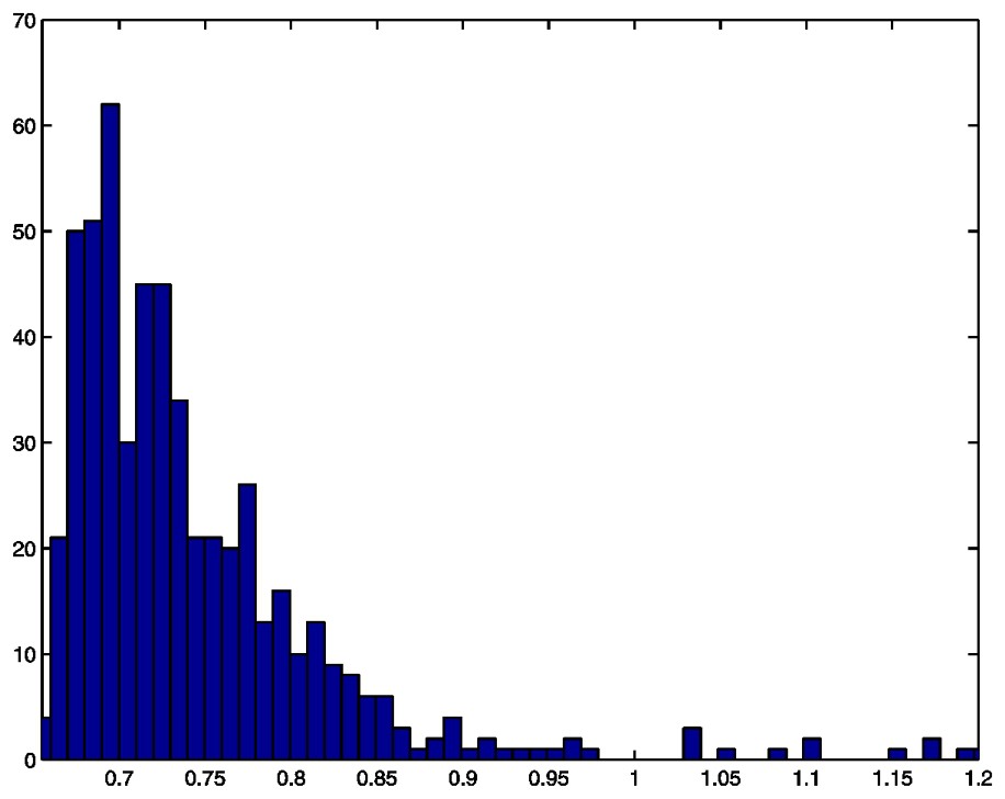
Histogram of cell masses, N=550.

5 Parameter estimation

5.1 Maximum likelihood method

We here discuss the estimation of model parameters from a sample of cell masses, specifically the sample illustrated in Fig. 1. We first assume that the model is given by (6), that is a three-parametric convolution of an exponential distribution with a Gaussian one. In the next section we allow occasional high masses, occurring with a probability δ, which is then an additional parameter to be estimated.

Let the sample be x1, x2, ‘Λ’, xN. The likelihood function is:

L(a,μ,σ)=i=1Nf(xi,a,μ,σ)
where
f(xi,a,μ,σ)=a exp a2σ22-a(xi-μ)Φxi-μ-σ2aσ(11)
The maximum likelihood estimates satisfy the likelihood equations:
log La=0, log Lμ=0, log Lσ=0
We have, taking natural logarithms,
log L(a,μ,σ)=N log a+Na2σ22-ai=1Nxi+ Na μ+i=1N log Φxi-μ-σ2aσ
and we obtain the following equations: (12)
where
zi=xi-μ-σ2aσ

These equations, which can be simplified, are expressed above in the form E(·|x1,…,xn)=E(·), for a representation of the minimal sufficient statistic of the ‘complete’ exponential family we would have had if we could have observed the exponential and the Gaussian separately. It is impossible to solve these equations explicitly, so some iterative method is required. One possibility is to use the EM algorithm [18,19], which will iterate between the left- and right-hand sides of (12), but it will be quite slow. Therefore, we instead eliminated μ (μ=x¯-1/a) from the first equation and obtained the following profile-likelihood function for (a,σ):

log L(a,σ)=N log a+ Na 2σ22- Na x¯+ Na x¯-1a+i=1N log Φxi-(x¯-1/a)-σ2aσ

We calculated the above log-likelihood function over a grid of different values of the parameters a and σ. The maximum point was found by making the grid successively finer. Based on the complete cell mass data shown in Fig. 1, the parameters were estimated to be: a=11.6, μ=0.6656, σ=0.0079. This estimated distribution did not fit the data well (solid line in Fig. 2).

Fig. 2

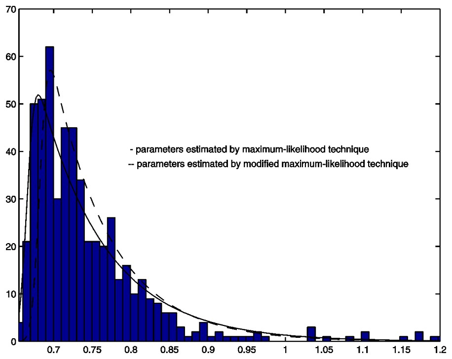
Histogram and two density functions.

5.2 Modified maximum-likelihood method

The following modified ML iterative procedure was found to be practical and adequate for dealing with the high cell masses in the large sample of data that was available (N=550). As the first step, model (6) is fitted by ML to all of data, as described above. In the fitted model, the (high) value t is determined such that only one observation should have been expected above t, according to (6). In our case, an explicit and close approximation to t is given by:

exp -a^(t-μ^)+a^2σ^2/2=1/N
because in the tail of (6) the Φ-factor will be close to 1. Now, all but one of the d (say) actual observations above t are assumed to represent what we call high losses, and consequently the probability δ for high losses can be estimated as δ^=(d-1)/N. If exactly one observation were to be found above t, its expected value in the fitted distribution would be approximately t+1/λ^. Hence, as the second step, the d actual observations above t are replaced by a single observation at t+1/λ^, and the parameters of (6) are re-estimated.

This procedure is repeated until convergence.

With the actual data shown in Fig. 1, the parameters were estimated to be: a=15.0, μ=0.6673, σ=0.0089. Fig. 2 shows the fit of this distribution to the data truncated at 1.05.

6 Generation times

In the previous sections, we considered the cell mass at division for models of the cell cycle. Knowing the distribution of birth masses, we can also determine the distribution of generation times, i.e. the time from cell birth to division. In the particular case when fn=f*(n=0,1,) is a time-independent stationary sequence, the distribution of generation time has the same property.

We tried to verify our convolution model using experimental data from mouse L. We received the data from Prof. Michael C. Mackey (McGill University, Montreal, Canada). The data contain 89 pairs of generation times for respective daughter (sister) cells. Using the maximum-likelihood technique described in Section 5.1, we estimate parameters in the convolution model to be: a=3.2, μ=0.5178, σ=0.02. The theoretical density function fits the experimental data quite well (see Fig. 3). The same experimental data (mouse L) was used before to check the sister cell model described in [12]. The fitting of the data by the density function in the convolution model is much better than it was in the sister cell model (see Fig. 4 in [12]).

Fig. 3

Histogram (experimental data) and density function estimated by maximum-likehood technique.

7 Conclusion

We have estimated the cell cycle models that have a mixture of deterministic and probabilistic dynamics. We proposed to estimate a distribution of cell birth masses with truncated convolution of Gaussian and exponential distributions. It was shown that our convolution model fits well both the Monte Carlo simulated data and experimental data (mouse L). It is very important to be able to calculate the probability that a cell mass exceeds some level. The ability to control a pathological growth has a big significance in the biology. The saddle-point approximation method presented here is very useful in calculating such tail probabilities. This method is good not only in our convolution model, but in many other possible models, since it gives good approximations to small tail probabilities.


Bibliographie

[1] T.E. Harris The Theory of Branching Processes, Springer, Berlin, 1963

[2] P. Jagers Branching Processes with Biological Applications, Wiley, 1975

[3] L. Glass; M.C. Mackey From Clocks to Chaos: The Rhytms of Life, Princeton University Press, Princeton, NJ, 1988

[4] A. Lasota; M.C. Mackey Globally asymptotic properties of proliferating cell populations, J. Math. Biol., Volume 19 (1984), pp. 43-62

[5] J.J. Tyson; K.B. Hannsgen Cell growth and division: a deterministic/probabilistic model of the cell cycle, J. Math. Biol., Volume 23 (1986), pp. 231-246

[6] K.B. Hannsgen; J.J. Tyson; L.T. Watson Steady-state size distributions in probabilistic models of the cell division cycle, SIAM J. Appl. Math., Volume 45 (1985) no. 4, pp. 523-540

[7] J.J. Tyson; K.B. Hannsgen Global asymptotic stability of the size distribution in probabilistic models of the cell cycle, J. Math. Biol., Volume 22 (1985), pp. 61-68

[8] J. Tyrcha Asymptotic stability in a generalized probabilistic/deterministic model of the cell cycle, J. Math. Biol., Volume 26 (1988), pp. 465-475

[9] A. Lasota; M.C. Mackey; J. Tyrcha The statistical dynamics of irregular biological events, J. Math. Biol., Volume 30 (1992), pp. 775-800

[10] J.A. Smith; L. Martin Do cells cycle?, Proc. Natl Acad. Sci. USA, Volume 70 (1973), pp. 1263-1267

[11] R. Shields Transition probability and the origin of variation in the cell cycle, Nature, Volume 267 (1977), pp. 704-707

[12] J. Tyrcha Age-dependent cell cycle models, J. Theor. Biol., Volume 213 (2001), pp. 89-101

[13] R. Sennerstam; J.-O. Strömberg Cell cycle progression: computer simulation of uncoupled subcycles of DNA replication and cell growth, J. Theor. Biol., Volume 175 (1995), pp. 177-189

[14] J.L. Jensen Saddlepoint Approximations, Oxford University Press, Oxford, UK, 1995

[15] J.E. Kolassa Series Approximation Methods in Statistics, Springer, New York, 1997

[16] J. Tyrcha; R. Sundberg; P. Lindskog; B. Sundström Statistical modelling and saddle-point approximation of tail probabilities for accumulated splice loss in fibre-optic networks, J. Appl. Stat., Volume 27 (2000) no. 2, pp. 245-256

[17] R. Sundberg Maximum likelihood theory for incomplete data from an exponential family, Scand. J. Stat., Volume 1 (1974), pp. 49-58

[18] A.P. Dempster; N.M. Laird; D.B. Rubin Maximum likelihood from incomplete data via EM algorithm (with discussion), J. R. Stat. Soc. Ser. B, Volume 39 (1977), pp. 1-38

[19] R. Sundberg An iterative method for solution of the likelihood equations for incomplete data from exponential families, Commun. Stat. B, Volume 5 (1976), pp. 55-64


Commentaires - Politique


Ces articles pourraient vous intéresser

Statistical analysis of oligonucleotide microarray data

Ziad Taib

C. R. Biol (2004)


Optimal calibration marker mesh for 2D X-ray sensors in 3D reconstruction

Laurent Desbat; Catherine Mennessier; Guillaume Champleboux

C. R. Biol (2002)


Models for pattern formation in somitogenesis: a marriage of cellular and molecular biology

Santiago Schnell; Philip K. Maini; Daragh McInerney; ...

C. R. Biol (2002)