Coexistence in competition models with density-dependent mortality

Shigui Ruan; Ada Ardito; Paolo Ricciardi; Don L. DeAngelis

doi:10.1016/j.crvi.2007.10.004

Biological modelling / Biomodélisation

Coexistence in competition models with density-dependent mortality
[Coexistence dans des modèles de compétition avec mortalité densité dépendante]

Présenté par : Pierre Auger

Shigui Ruan ¹ ; Ada Ardito ² ; Paolo Ricciardi ² ; Don L. DeAngelis ³

¹ Department of Mathematics, University of Miami, P.O. Box 249085, Coral Gables, FL 33124-4250, USA
² Dipartimento di Matematica, Universitá di Roma “La Sapienza”, P. le Aldo Moro, 2, 00185 Roma, Italy
³ Department of Biology, University of Miami, P.O. Box 249118, Coral Gables, FL 33124-0421, USA

Comptes Rendus. Biologies, Volume 330 (2007) no. 12, pp. 845-854.

Résumés

Anglais
Français

We consider a two-competitor/one-prey model in which both competitors exhibit a general functional response and one of the competitors exhibits a density-dependent mortality rate. It is shown that the two competitors can coexist upon the single prey. As an example, we consider a two-competitor/one-prey model with a Holling II functional response. Our results demonstrate that density-dependent mortality in one of the competitors can prevent competitive exclusion. Moreover, by constructing a Liapunov function, the system has a globally stable positive equilibrium.

Nous considérons un modèle à deux compétiteurs et une proie, dans lequel les deux compétiteurs ont une réponse fonctionnelle générale et un des compétiteurs possède un taux de mortalité densité dépendant. Nous montrons que les deux compétiteurs peuvent coexister en présence d'une seule proie. Pour illustrer nos résultats, nous considérons un modèle deux compétiteurs/une proie avec une réponse fonctionnelle de type Holling II. Ces résultats prouvent qu'un taux de mortalité densité dépendant chez un des compétiteurs peut empécher l'exclusion compétitive. De plus, en construisant une fonction de Lyapunov, nous montrons que le système possède un équilibre positif globalement stable.

Métadonnées

Reçu le : 2007-07-12
Accepté le : 2007-10-03
Publié le : 2007-11-07

PMID

DOI : 10.1016/j.crvi.2007.10.004

Keywords: Competition, Functional response, Density-dependent mortality, Competitive exclusion, Coexistence
Mot clés : Compétition, Réponse fonctionnelle, Mortalité densité dépendante, Exclusion compétitive, Coexistence

Affiliations des auteurs :

Shigui Ruan ¹ ; Ada Ardito ² ; Paolo Ricciardi ² ; Don L. DeAngelis ³

@article{CRBIOL_2007__330_12_845_0,
     author = {Shigui Ruan and Ada Ardito and Paolo Ricciardi and Don L. DeAngelis},
     title = {Coexistence in competition models with density-dependent mortality},
     journal = {Comptes Rendus. Biologies},
     pages = {845--854},
     publisher = {Elsevier},
     volume = {330},
     number = {12},
     year = {2007},
     doi = {10.1016/j.crvi.2007.10.004},
     language = {en},
}

TY  - JOUR
AU  - Shigui Ruan
AU  - Ada Ardito
AU  - Paolo Ricciardi
AU  - Don L. DeAngelis
TI  - Coexistence in competition models with density-dependent mortality
JO  - Comptes Rendus. Biologies
PY  - 2007
SP  - 845
EP  - 854
VL  - 330
IS  - 12
PB  - Elsevier
DO  - 10.1016/j.crvi.2007.10.004
LA  - en
ID  - CRBIOL_2007__330_12_845_0
ER  -

%0 Journal Article
%A Shigui Ruan
%A Ada Ardito
%A Paolo Ricciardi
%A Don L. DeAngelis
%T Coexistence in competition models with density-dependent mortality
%J Comptes Rendus. Biologies
%D 2007
%P 845-854
%V 330
%N 12
%I Elsevier
%R 10.1016/j.crvi.2007.10.004
%G en
%F CRBIOL_2007__330_12_845_0

Shigui Ruan; Ada Ardito; Paolo Ricciardi; Don L. DeAngelis. Coexistence in competition models with density-dependent mortality. Comptes Rendus. Biologies, Volume 330 (2007) no. 12, pp. 845-854. doi : 10.1016/j.crvi.2007.10.004. https://comptes-rendus.academie-sciences.fr/biologies/articles/10.1016/j.crvi.2007.10.004/

Version originale du texte intégral

1 Introduction

The principle of competitive exclusion [13,17,20,35,47] asserts that two or more competitors cannot coexist indefinitely on a single prey, which was supported by experiments on Paramecium cultures by Gause [15] (see also [28]). It was thought to hold in laboratory settings until Ayala [2] demonstrated experimentally that two species of Drosophila could coexist upon a single prey.

In order to explain Ayala's experiments, various competition models have been proposed. For example, Armstrong and McGehee [1] considered the model:

(1.1)

where v and w are the densities of the two competitors and u is the density of the prey. In model (1.1) the contributions of the interaction between the competitor with density w and the prey u to the growth rates of those species are described by Holling II functional response terms. However, predation of a common prey is the only interaction between species v and w that is represented. Armstrong and McGehee [1,36] found that, for appropriate parameter values and suitable initial population densities

(u (0), v (0), w (0))

, system (1.1) does predict the coexistence of the two competitors via a locally attracting periodic orbit. Hsu, Hubbell and Waltman [23,24] generalized this type of coexistence to the case when both competitors exhibit Holling II functional response (see also Butler and Waltman [4], Cushing [9], Farkas [12], Muratori and Rinaldi [37], Smith [41], etc.), i.e., to a system of the form:

(1.2)

These studies support Hutchinson's point [26] that the two competitive species “might oscillate in varying numbers, but persist almost indefinitely”. However, such systems do not possess a componentwise positive equilibrium [34] and thus no stable equilibrium is possible [31]. Moreover, system (1.2), exhibiting Armstrong- and McGehee-type coexistence is only weakly persistent, but not persistent. Hence, it is not permanent, otherwise it would exhibit componentwise positive equilibria (see [27]).

Consider an ordinary differential equation model for n interacting biological species:

\frac{d u_{i}}{d t} = u_{i} f_{i} (u_{1}, u_{2}, \dots, u_{n}), i = 1, 2, \dots, n

(1.3)

where

u_{i} (t)

denotes the density of the ith species. Let

(u_{1} (t), u_{2} (t), \dots, u_{n} (t))

denote the solution of system (1.3), with componentwise positive initial values. The system (1.3) is said to be weakly persistent if:

\underset{t \to \infty}{lim sup} u_{i} (t) > 0, i = 1, 2, \dots, n

persistent if:

\underset{t \to \infty}{lim inf} u_{i} (t) > 0, i = 1, 2, \dots, n

and uniformly persistent if there is an

ε_{0} > 0

such that

\underset{t \to \infty}{lim inf} u_{i} (t) ⩾ ε_{0}, i = 1, 2, \dots, n

The system (1.3) is said to be permanent if, for each

i = 1, 2, \dots, n

, there are constants

ε_{i}

and

M_{i}

such that:

0 < ε_{i} ⩽ \underset{t \to \infty}{lim inf} u_{i} (t) ⩽ \underset{t \to \infty}{lim sup} u_{i} (t) ⩽ M_{i}

Clearly, permanence implies uniform persistence, which in turn implies persistence, and persistence implies weak persistence; a dissipative uniformly persistent system is permanent. For further discussion about various definitions of persistence and permanence and their connections, we refer to [14,27,43,48].

To have the strong version of coexistence, researchers have taken various other factors into account when modeling competition, such as interspecific interference [45,46], spatial heterogeneity [5], stoichiometric principles [34], etc. Another important factor is intraspecific interference within a population of competitors, which includes aggressive displays, posturing, fighting, infanticide, and cannibalism [30]. When the principal effect of the intraspecific interference is a reduced rate of feeding or resource intake, the effects can be modeled via an altered functional response for the consumer [8,10,40]. Recently, Cantrell et al. [6] extended system (1.2) to incorporate conspecific feeding interference for one of the competitors. The functional responses for the competitor w and the prey u are now taken to have the Beddington–DeAngelis form:

\frac{E u}{1 + B u + C w}

where Cw may be viewed as accounting for mutual feeding interference among members of the competitors. It was demonstrated that two competitors not only coexist upon a single prey in the sense of uniform persistence, but also have a globally stable equilibrium.

On the other hand, when lethal fighting or cannibalism occurs, it is more appropriate to include a nonlinear (density-dependent) mortality term for the consumer into the competition model [30]. In plant population, density-dependent mortality is one of the three principal effects resulting from intraspecific competition [38,49]. To incorporate such intraspecific competition (as well as the interspecific competition) into the model, Ruan and He [39] studied the global stability of a chemostat-type competition model, Kuang et al. [30] investigated the global stability of a Lotka–Volterra competition model. See also [16,32,33] for persistence of n species on a single resource.

Notice that in Refs. [16,30,32,33,39] all competitors are assumed to have density-dependent mortality rates. A very natural and very significant question arises: If one of the competitors does not have a density-dependent mortality rate, does the model still exhibit coexistence and have a stable componentwise positive equilibrium? The numerical simulations of Kuang et al. [30] indicate that, even for a Lotka–Volterra model, a competitor without a density-dependent mortality rate could eliminate another competitor with a density-dependent mortality rate if the first competitor has a lower break-even prey biomass. The problem can be very subtle.

Hixon and Jones [21] found that density-dependent mortality in demersal marine fishes is often caused by the interplay of predation and competition (see also [22]). To study how the nonlinear mortality rate determines the dynamics of such competition models qualitatively, we consider a two-competitor/one-prey model of the form:

(1.4)

under the initial value conditions:

(1.5)

The functional responses for the predators v and w are given by

f (u)

and

g (u)

, respectively, which are increasing and continuously differentiable functions,

f (0) = g (0) = 0

. The density-dependent mortality term for the second species,

G w^{2}

, also referred to as a ‘closure term’, describes either a self-limitation of the consumers, w, or the influence of predation (see [42] and [29]). Self-limitation can occur if another factor besides food can possibly become limiting at high population densities. Predation on consumers can increase as the

w^{2}

power if higher consumer densities attract greater attention from predators or if consumers become more vulnerable at higher densities. Zooplankton, for example, can experience density-dependent mortality when population densities are high (see [7,11,39,42]).

We shall show that the two competitors can coexist upon the single prey. It demonstrates that density-dependent mortality in one of the competitors can prevent competitive exclusion.

As an example, we apply the obtained results to a two-competitor/one-prey model with a Holling II functional response:

(1.6)

More specific conditions on local and global stability are given in terms of the model parameters. Model (1.6) differs from model (1.2) in an important respect. The growth of species w in (1.6) is strictly limited, due to the

G w^{2}

term, and can become non-positive for large enough values of w, no matter what the size of its prey, u, is. In model (1.2), it is always possible for the prey density, u, to be large enough for the growth rate of w to be positive. Thus, model (1.6) differs significantly from the others and warrants separate investigation.

2 Mathematical analysis

2.1 General functional responses

First of all, we can see that the solutions to the initial value problem (1.4)–(1.5) are nonnegative.

Define $U (t) = u + \frac{a}{e} v + \frac{A}{E} w$ and denote $d_{0} = \min {d, D}$ . We have:

\frac{d U}{d t} ⩽ (r + d_{0}) (K + ε) - d_{0} U

where

ε > 0

. The comparison principle implies that the solutions of system (1.4) are bounded.

Next, we consider the existence of a positive equilibrium. System (1.4) has a componentwise positive equilibrium $E^{*} = (u^{*}, v^{*}, w^{*})$ , where:

(2.1)

if:

r u^{*} (1 - \frac{u^{*}}{K}) - A w^{*} g (u^{*}) > 0

(2.2)

and

G > 0, E g (u^{*}) - D > 0

(2.3)

It is important to note that the key assumption for the existence of the positive equilibrium $E^{*}$ is $G > 0$ . If $G = 0$ , then the positive equilibrium simply does not exist. To have $w^{*} > 0$ , we require $E g (u^{*}) > D$ , which means that at the steady state the growth rate of the species w must be greater than the linear mortality rate. Notice that from the first equation, we have:

r u^{*} (1 - \frac{u^{*}}{K}) - a v^{*} f (u^{*}) - A w^{*} g (u^{*}) = 0

which gives:

a v^{*} f (u^{*}) = r u^{*} (1 - \frac{u^{*}}{K}) - A w^{*} g (u^{*}) > 0

v^{*} > 0

is well defined.

Now we study the local stability of the positive equilibrium $E^{*}$ . Define:

ρ (u) = \frac{r}{K} + a v^{*} {(\frac{f (u)}{u})}^{'} + A w^{*} {(\frac{g (u)}{u})}^{'}

(2.4)

The Jacobian matrix of system (1.4) at

E^{*}

takes the form:

J^{*} = [\begin{matrix} j_{11} & j_{12} & j_{13} \\ j_{21} & 0 & 0 \\ j_{31} & 0 & j_{33} \end{matrix}]

(2.5)

where:

j_{11} = - u^{*} ρ (u^{*})

j_{12} = - a f (u^{*}) < 0

j_{13} = - A g (u^{*}) < 0

j_{21} = e v^{*} f^{'} (u^{*}) > 0

j_{31} = E w^{*} g^{'} (u^{*}) > 0

j_{33} = - G w^{*} < 0

The positive equilibrium

E^{*}

is locally stable if all eigenvalues of the Jacobian matrix

J^{*}

given by (2.5) have negative real parts. The characteristic equation is given by:

λ^{3} + a_{1} λ^{2} + a_{2} λ + a_{3} = 0

(2.6)

where

a_{1} = - (j_{11} + j_{33}) = u^{*} ρ (u^{*}) + G w^{*}

a_{2} = j_{11} j_{33} - j_{13} j_{31} - j_{12} j_{21}

a_{3} = j_{12} j_{21} j_{33} = a e G v^{*} w^{*} f (u^{*}) f^{'} (u^{*}) > 0

Routh–Hurwitz criteria state that all roots of the characteristic equation (2.6) have negative real parts if:

a_{1} > 0, a_{3} > 0, a_{1} a_{2} - a_{3} > 0

Since $a_{3} > 0$ , the characteristic equation (2.6) always has at least one negative real root. Notice that:

a_{1} a_{2} - a_{3} = G {(u^{*})}^{2} w^{*} T (ρ (u^{*}))

where:

T (ρ (u^{*})) = ρ {(u^{*})}^{2} + ρ (u^{*}) [\frac{a e v^{*}}{G w^{*}} \frac{f (u^{*})}{u^{*}} f^{'} (u^{*}) + \frac{A E}{G} \frac{g (u^{*})}{u^{*}} g^{'} (u^{*}) + \frac{G w^{*}}{u^{*}}] + \frac{A E w^{*}}{u^{*}} \frac{g (u^{*})}{u^{*}} g^{'} (u^{*})

Thus, we have

(i) $a_{1} > 0$ iff $u^{*} ρ (u^{*}) + G w^{*} > 0$
(ii) $a_{1} a_{2} - a_{3} > 0$ iff $T (ρ (u^{*})) > 0$

Observe that for the quadratic form

T (ρ (u^{*}))

, we have

Δ_{T} : = {[\frac{a e v^{*}}{G w^{*}} \frac{f (u^{*})}{u^{*}} f^{'} (u^{*})]}^{2} + 2 \frac{a e v^{*}}{G w^{*}} \frac{f (u^{*})}{u^{*}} f^{'} (u^{*}) [\frac{A E}{G} \frac{g (u^{*})}{u^{*}} g^{'} (u^{*}) + \frac{G w^{*}}{u^{*}}] + {[\frac{A E w^{*}}{u^{*}} \frac{g (u^{*})}{u^{*}} g^{'} (u^{*}) - \frac{G w^{*}}{u^{*}}]}^{2} > 0

(2.7)

and

T (- \frac{G w^{*}}{u^{*}}) = - \frac{a e v^{*}}{G w^{*}} \frac{f (u^{*})}{u^{*}} f^{'} (u^{*}) < 0

Thus

ρ_{+}^{*} > - \frac{G w^{*}}{u^{*}}

where

ρ_{+}^{*} = \frac{1}{2} {- [\frac{a e v^{*}}{G w^{*}} \frac{f (u^{*})}{u^{*}} f^{'} (u^{*}) + \frac{A E}{G} \frac{g (u^{*})}{u^{*}} g^{'} (u^{*}) + \frac{G w^{*}}{u^{*}}] + \sqrt{Δ_{T}}}

(2.8)

It follows that

a_{1} a_{2} - a_{3} > 0

iff

ρ (u^{*}) > ρ_{+}^{*}

. We observe that

ρ_{+}^{*} < 0

. Therefore, by Routh–Hurwitz criteria we have the following result on the local stability of

E^{*}

Theorem 2.1

Assume that the positive equilibrium $E^{*}$ exists. If

u^{*} ρ (u^{*}) + G w^{*} > 0

(2.9)

and

ρ (u^{*}) > ρ_{+}^{*}

(2.10)

then it is locally asymptotically stable.

Remark 2.2

The conditions (2.9) and (2.10) (corresponding (2.17) and (2.18) in Proposition 2.4) are technical assumptions on parameters. For the specific Holling II functional response, these conditions will be expressed explicitly, see Remark 2.7. Also, since $ρ_{+}^{*} < 0$ , we can see that $ρ (u^{*}) > 0$ implies both (2.9) and (2.10). Thus, conditions (2.9) and (2.10) can be replaced by a stronger condition

ρ (u^{*}) > 0

Remark 2.3

Assume $ρ (u^{*}) = ρ_{+}^{*}$ for certain parameter value, say a critical value of the carrying capacity of the prey population, $K = K_{c}$ . Then the characteristic equation (2.6) has a pair of purely imaginary roots given by $λ_{2, 3} = \pm i \sqrt{a_{2}}$ . If, moreover, the transversality condition

\frac{d}{d K} λ_{2, 3} (K) |_{K = K_{c}} > 0

holds, then the positive equilibrium

E^{*}

becomes unstable and a Hopf bifurcation occurs at

E^{*}

when K passes through

K_{c}

Finally, we discuss the global stability of the positive equilibrium $E^{*}$ . Choose a Liapunov function as follows:

V (u, v, w) = α \int_{u^{*}}^{u} \frac{x - u^{*}}{x} d x + β \int_{v^{*}}^{v} \frac{y - v^{*}}{y} d y + γ \int_{w^{*}}^{w} \frac{z - w^{*}}{z} d z,

(2.11)

where α, β, and γ are positive constants to be determined. Along any trajectory of system (1.4), we have:

\frac{d V}{d t} = α (u - u^{*}) [r (1 - \frac{u}{K}) - a v \frac{f (u)}{u} - A w \frac{g (u)}{u}] + β (v - v^{*}) [- d + e f (u)] + γ (w - w^{*}) [- D - G w + E g (u)] = α (u - u^{*}) [- \frac{r (u - u^{*})}{K} - a v^{*} (\frac{f (u)}{u} - \frac{f (u^{*})}{u^{*}}) - A w^{*} (\frac{g (u)}{u} - \frac{g (u^{*})}{u^{*}}) - a \frac{f (u)}{u} (v - v^{*}) - A \frac{g (u)}{u} (w - w^{*})]

Define:

ϕ_{1} (ξ_{1} u) = {\frac{d}{d u} (\frac{f (u)}{u}) |}_{u = ξ_{1} u}, 0 < ξ_{1} < 1

ϕ_{2} (ξ_{2} u) = {\frac{d}{d u} (\frac{g (u)}{u}) |}_{u = ξ_{2} u}, 0 < ξ_{2} < 1

so that:

\frac{f (u)}{u} - \frac{f (u^{*})}{u^{*}} = ϕ_{1} (ξ_{1} u) (u - u^{*})

\frac{g (u)}{u} - \frac{g (u^{*})}{u^{*}} = ϕ_{2} (ξ_{2} u) (u - u^{*})

Also, denote:

f (u) - f (u^{*}) = f^{'} (ξ_{3} u) (u - u^{*}), 0 < ξ_{3} < 1

g (u) - g (u^{*}) = g^{'} (ξ_{4} u) (u - u^{*}), 0 < ξ_{4} < 1

Therefore, we have:

\frac{d V}{d t} = α [- \frac{r}{K} - a v^{*} ϕ_{1} (ξ_{1} u) - A w^{*} ϕ_{2} (ξ_{2} u)] {(u - u^{*})}^{2} + [α a \frac{f (u)}{u} + β e f^{'} (ξ_{3} u)] (u - u^{*}) (v - v^{*}) + [α A \frac{g (u)}{u} + γ E g^{'} (ξ_{4} u)] (u - u^{*}) (w - w^{*}) - γ G {(w - w^{*})}^{2} = z S z^{T}

where

z = (u - v^{*}, v - v^{*}, w - w^{*})

and the matrix

S = {(s_{i j})}_{3 \times 3}

is defined as

s_{11} = α [- \frac{r}{K} - a v^{*} ϕ_{1} (ξ_{1} u) - A w^{*} ϕ_{2} (ξ_{2} u)]

s_{12} = s_{21} = \frac{1}{2} [α a \frac{f (u)}{u} + β e f^{'} (ξ_{3} u)]

s_{13} = s_{31} = \frac{1}{2} [α A \frac{g (u)}{u} + γ E g^{'} (ξ_{4} u)]

s_{22} = s_{23} = s_{32} = 0, s_{33} = - γ G

If α, β and γ can be chosen suitably such that S is negative definite for all

(u, v, w) \in R_{+}^{3}

, then

\frac{d V}{d t} ⩽ 0

and

\frac{d V}{d t} = 0

if and only if

u = u^{*}

v = v^{*}

w = w^{*}

. The largest invariant subset of the set of the points where

\frac{d V}{d t} = 0

(u^{*}, v^{*}, w^{*})

. Therefore, LaSalle's Invariance Principle implies that

E^{*} = (u^{*}, v^{*}, w^{*})

is globally stable.

In next subsection, for the model with Holling II functional responses, we will choose proper $α, β$ and γ to derive explicit sufficient conditions for the global stability of the positive equilibrium.

2.2 Holling II functional responses

In this subsection we apply the above results to system (1.4) with Holling II functional responses, namely system (1.6). System (1.6) has a unique componentwise positive equilibrium $E^{*} = (u^{*}, v^{*}, w^{*})$ defined by:

u^{*} = \frac{d}{e - b d} v^{*} = \frac{1 + b u^{*}}{a} [r (1 - \frac{u^{*}}{K}) - \frac{A w^{*}}{1 + B u^{*}}] w^{*} = \frac{1}{G} (- D + \frac{E u^{*}}{1 + B u^{*}}) = \frac{1}{G} (- D + \frac{E d}{B d + e - b d})

(2.12)

provided

r (1 - \frac{u^{*}}{K}) - \frac{A w^{*}}{1 + B u^{*}} > 0

(2.13)

and

G > 0, \frac{e}{b} > d, \frac{E d}{B d + e - b d} > D

(2.14)

Note that the last two inequalities in (2.14) simply mean that the death rates of the two competitors must be smaller than the corresponding growth rates, otherwise the competing species cannot survive and the positive steady state does not exist.

Define

ρ_{1} (u) = \frac{r}{K} - \frac{a b v^{*}}{(1 + b u) (1 + b u^{*})} - \frac{A B w^{*}}{(1 + B u) (1 + B u^{*})}

(2.15)

We have:

T (ρ_{1} (u^{*})) = ρ_{1} {(u^{*})}^{2} + ρ_{1} (u^{*}) [\frac{e a v^{*}}{G w^{*} {(1 + b u^{*})}^{3}} + \frac{E A}{G {(1 + B u^{*})}^{3}} + \frac{G w^{*}}{u^{*}}] + \frac{E A w^{*}}{u^{*} {(1 + B u^{*})}^{3}}

Δ_{T} : = {[\frac{v^{*}}{w^{*}} \frac{e a}{G {(1 + b u^{*})}^{3}}]}^{2} + \frac{2 e a v^{*}}{G w^{*} {(1 + b u^{*})}^{3}} [\frac{E A}{G {(1 + B u^{*})}^{3}} + \frac{G w^{*}}{u^{*}}] + {[\frac{E A}{G {(1 + B u^{*})}^{3}} - \frac{G w^{*}}{u^{*}}]}^{2} > 0

and

ρ_{1}^{*} = \frac{1}{2} {- [\frac{e a v^{*}}{G w^{*} {(1 + b u^{*})}^{3}} + \frac{E A}{G {(1 + B u^{*})}^{3}} + \frac{G w^{*}}{u^{*}}] + \sqrt{Δ_{T}}}

(2.16)

By Theorem 2.1, we have the following local stability result.

Proposition 2.4

Assume that the positive equilibrium $E^{*}$ of system (1.6) exists. If

u^{*} ρ_{1} (u^{*}) + G w^{*} > 0

(2.17)

and

ρ_{1} (u^{*}) > ρ_{1}^{*}

(2.18)

then it is locally stable.

Remark 2.5

Note that $ρ (u^{*})$ , defined by Eq. (2.4), is for general functional responses, while $ρ_{1} (u^{*})$ , defined by Eq. (2.15), is for the specific Holling type-II functional response. They both are related to the derivative of the right-hand side function of the prey equation, that is, the growth of the prey population at the positive equilibrium.

Finally, we give a sufficient condition for the global stability of the positive equilibrium $E^{*}$ for system (1.6).

Proposition 2.6

Assume that the positive equilibrium $E^{*}$ of system (1.6) is locally stable. If

ρ_{1} (0) > 0

(2.19)

then it is globally stable.

Proof

Let $V (u, v, w)$ be the Liapunov function defined by (2.11), where α, β, and γ are positive constants to be determined. Along any trajectory of system (1.6), we have:

\frac{d V}{d t} = α [- \frac{r}{K} + \frac{a b v^{*}}{(1 + b u) (1 + b u^{*})} + \frac{A B w^{*}}{(1 + B u) (1 + B u^{*})}] {(u - u^{*})}^{2} + \frac{1}{1 + b u} [- α a + β e - \frac{β b e u^{*}}{1 + b u^{*}}] (u - u^{*}) (v - v^{*}) + \frac{1}{1 + B u^{*}} [- α A + γ E - \frac{γ B E u^{*}}{1 + B u^{*}}] (u - u^{*}) (w - w^{*}) - γ G {(w - w^{*})}^{2}

Choose

α = 1, β = \frac{a}{e - b d}

γ = \frac{A (e - b d + B d)}{E (e - b d)}

Then we have

\frac{d V}{d t} = [- \frac{r}{K} + \frac{a b v^{*}}{(1 + b u) (1 + b u^{*})} + \frac{A B w^{*}}{(1 + B u) (1 + B u^{*})}] {(u - u^{*})}^{2} - \frac{A G (e - b d + B d)}{E (e - b d)} {(w - w^{*})}^{2}

The coefficient for

{(w - w^{*})}^{2}

is always negative. The coefficient for

{(u - u^{*})}^{2}

is:

- ρ_{1} (u) = - \frac{r}{K} + \frac{a b v^{*}}{(1 + b u) (1 + b u^{*})} + \frac{A B w^{*}}{(1 + B u) (1 + B u^{*})} ⩽ - \frac{r}{K} + \frac{a b v^{*}}{1 + b u^{*}} + \frac{A B w^{*}}{1 + B u^{*}} ⩽ - ρ_{1} (0)

Thus, if (2.19) is satisfied, then

\frac{d V}{d t} ⩽ 0

and

\frac{d V}{d t} = 0

if and only if

u = u^{*}

v = v^{*}

w = w^{*}

. This completes the proof. □

Remark 2.7

Using (2.12), (2.15) and (2.19), one of the local stability conditions (2.17) becomes:

u^{*} [\frac{r}{K} - \frac{a b v^{*}}{{(1 + b u^{*})}^{2}} - \frac{A B w^{*}}{{(1 + B u^{*})}^{2}}] + G w^{*} > 0

(2.20)

and the global stability condition (2.19) reduces to

K < \frac{d + e - b d}{e - b d}

(2.21)

We can see that G plays a role in the local stability condition (2.20). Once the positive equilibrium is locally stable, K, the carrying capacity of the prey, plays a role in the global stability. If the value of K is increased so that condition (2.21) is not satisfied, the positive equilibrium becomes unstable and a Hopf bifurcation can occur (see Figs. 4 and 5).

Fig. 4
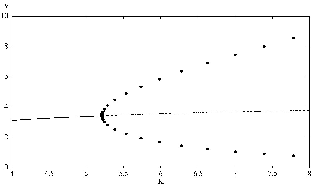
The bifurcation diagram shows that the positive equilibrium is stable when K⩽5.21. At K=5.21, it loses its stability and a supercritical Hopf bifurcation occurs. Here r=1.5, a=0.45, b=0.35, d=0.45, e=0.55, A=0.55, B=0.35, D=0.45, E=0.65, G=0.1. XPPAUT was used for the simulations.

Fig. 5
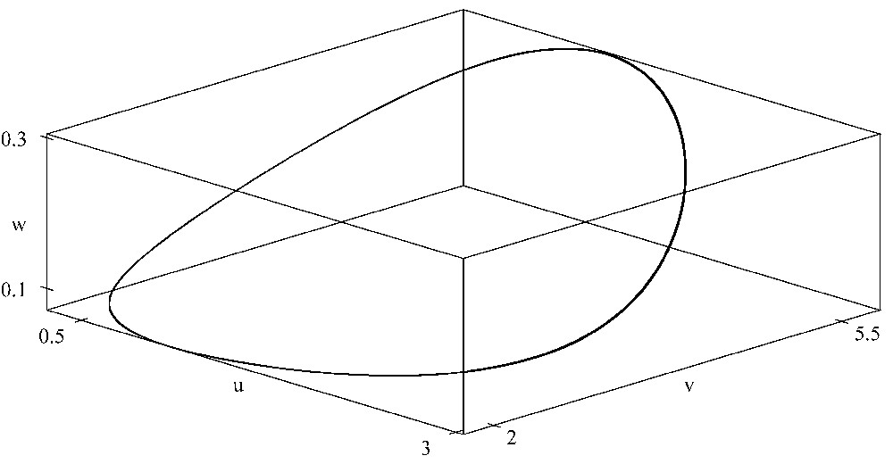
When K=6, there is a periodic orbit bifurcated from the interior equilibrium in the three-dimensional space which is asymptotically stable. Here r=1.5, a=0.45, b=0.35, d=0.45, e=0.55, A=0.55, B=0.35, D=0.45, E=0.65, G=0.1. XPPAUT was used for the simulations.

The plot of $ρ_{1} (u)$ indicates that $ρ_{1} (0) > 0$ for some parameter values (see Fig. 1). So the assumption $ρ_{1} (0) > 0$ in Theorem 2.6 makes sense.

Fig. 1
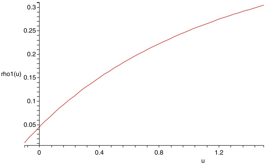
The plot of the function $ρ_{1} (u)$ . Here r=1.5, K=3, a=0.45, b=0.35, d=0.45, e=0.55, A=0.55, B=0.35, D=0.45, E=0.65, and G=0.05.

3 Simulations and discussion

It is well known that density-dependent mortality terms (closure terms) can greatly affect the outcome of plankton models [42]: not only limit cycles [11] but also chaos [7] can occur in such models.

In the case of two competitors competing for a common prey, our results indicate that density-dependent mortality of one competitor not only ensures the long-term survival of itself, but also guarantees the existence of the other competitor, which would otherwise be out-competed.

To illustrate the results numerically, consider system (1.6) with Holling II functional responses. Choose $r = 1.5$ , $K = 3$ , $a = 0.45$ , $b = 0.35$ , $d = 0.45$ , $e = 0.55$ , $A = 0.55$ , $B = 0.35$ , $D = 0.45$ , $E = 0.65$ , and let G (the density-dependent mortality parameter) vary. When $G = 0$ , that is, when there is only linear mortality for the competitor with density w, numerical simulations show that the competitor with density w out-competes the competitor with density v (see Fig. 2). Note that system (1.6) does not have any positive equilibrium when $G = 0$ .

Fig. 2
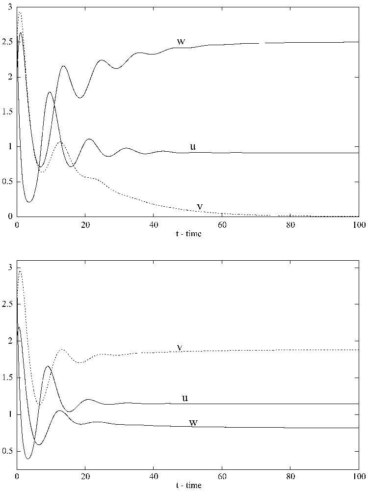
When G=0, the strong competitor with density w wins the competition and the weak competitor with density v tends toward extinction (top). When G=0.1, both competitors coexist and the solution converges to the positive equilibrium (1.1465,1.8837,0.8197) (bottom). XPPAUT was used for the simulations.

Introducing density-dependent mortality only for the competitor with density w (the stronger competitor) makes the system coexistent not only in the sense of uniform persistence, but also in the sense of existence of a globally stable positive equilibrium (Fig. 2). With the above parameter values and $G = 0.1$ , all conditions in Proposition 2.6 are satisfied. Thus, system (1.6) has a positive equilibrium $(1.1465, 1.8837, 0.8197)$ , which is globally stable. A possible explanation for this phenomenon is that density-dependent mortality in the stronger competitor prevents it from reducing the density of the prey below the threshold value (the $R^{*}$ value – see [44]) needed for the weaker competitor to be able to maintain itself. In fact, the steady-state values of v and w are functions of G (see Fig. 3).

Fig. 3
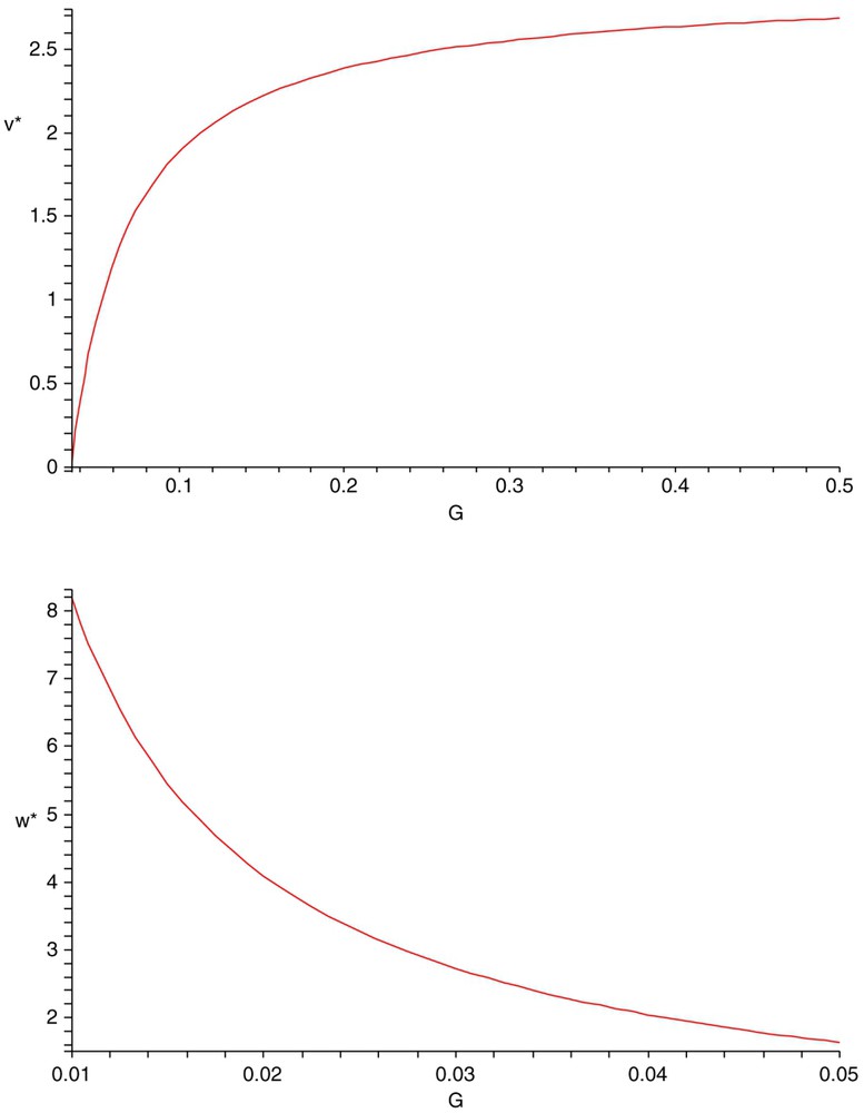
The steady-state value of the weak competitor with density v is an increasing function of G (top) and the steady-state value of the strong competitor with density w is a decreasing function of G (bottom). Here r=1.5, K=3, a=0.45, b=0.35, d=0.45, e=0.55, A=0.55, B=0.35, D=0.45, E=0.65.

Is the situation represented by model (1.4) a feasible one ecologically? It is a variation on the model of Tilman [44] for two consumers competing exploitatively for a single prey. Tilman's model predicts that the consumer that reduces the prey to the lower steady-state value will displace the other competitor. Model (1.4) includes the mechanism of density-dependent mortality, or biomass loss, $G w^{2}$ , on the superior competitor. We believe that this represents one way in which a fitness ‘tradeoff’ might occur between two species. It is reasonable to suppose that one species, w in this case, has superior fitness in its ability to exploit prey, but this is compensated for by a vulnerability to mortality. Increased mortality could reasonably occur under the circumstance that the superior competitor is also the one that is more of a risk taker; for example, that it seeks prey in areas where there is also a greater risk of mortality, say through predation. However, the non-linear form of the mortality, $G w^{2}$ , still requires justification. A nonlinear response of this form might occur if the foraging area contains a diversity of subareas having different relative risk factors. In that case, individuals of species w can tend to use areas that are relatively low in predation or other mortality risk (although higher than members of species v) when the population of species w is low, but can be forced into areas of higher risk as the population size increases. This situation could easily lead the better competitor to have also a density-dependent mortality rate. This might also occur if the better competitor is more prone to dispersal; the probability of dispersal of individuals increases with density, and dispersal increases the chances of mortality. Therefore, we believe that model (1.4) may represent a fairly common situation among consumers competing for a common prey.

It is interesting to observe that, when the carrying capacity K of the prey is increased, the positive equilibrium loses its stability and a Hopf bifurcation occurs when K passes a critical value. With parameters given above, a supercritical Hopf bifurcation occurs when $K = 5.21$ (see Fig. 4). A three-dimensional positive periodic solution bifurcates from the positive equilibrium via a Hopf bifurcation with $K = 6$ (see Fig. 5). This is an example of the well-known paradox of enrichment [25].

It is also interesting to notice that, for the subsystem without the competitor v, that is, the predator-prey system with density-dependent mortality:

\frac{d u}{d t} = r u (1 - \frac{u}{K}) - \frac{A u w}{1 + B u} \frac{d w}{d t} = w (- D - G w + \frac{E u}{1 + B u})

(3.1)

it is well known that (Bazykin [3], Hainzl [18,19]) very complex dynamics, such as the existence of multiple equilibria and multiple limit cycles, Hopf, homoclinc and Bagdanov–Takens bifurcations, can occur. Note that when system (1.6) has one positive equilibrium, it is unique. Thus, it does not exhibit complex dynamics as the 2-dimensional system (3.1) has. Our results indicate that introducing a weak competitor v (without density-dependent mortality) into the system has a stabilizing effect on the system, since the competition model (1.6) either has a globally stable positive equilibrium under certain conditions or exhibits the coexistence of both competitors in terms of positive periodic solutions.

Acknowledgements

The authors are very grateful to the anonymous referee for his careful reading, detailed comments, and helpful suggestions. The first author would like to thank Prof. G. Bard Ermentrout and Dr. Rongsong Liu for their help in using XPPAUT for the numerical simulations.

Bibliographie

[1] R.A. Armstrong; R. McGehee Competitive exclusion, Am. Nat., Volume 115 (1980), pp. 151-170

[2] F.J. Ayala Experimental invalidation of the principle of competitive exclusion, Nature, Volume 224 (1969), pp. 1076-1079

[3] A.D. Bazykin Nonlinear Dynamics of Interacting Populations, World Scientific, Singapore, 1998

[4] G.J. Butler; P. Waltman Bifurcation from a limit cycle in a two predator-one prey ecosystem modeled on a chemostat, J. Math. Biol., Volume 12 (1981), pp. 295-310

[5] R.S. Cantrell; C. Cosner Spatial Ecology via Reaction–Diffusion Equations, Series in Math. Comput. Biol., John Wiley and Sons, Chichester, UK, 2003

[6] R.S. Cantrell; C. Cosner; S. Ruan Intraspecific interference and consumer-resource dynamics, Dis. Con. Dynam. Syst., Volume 4B (2004), pp. 527-546

[7] H. Caswell; M.G. Neubert Chaos and closure terms in plankton food chain models, J. Plankton Res., Volume 20 (1998), pp. 1837-1845

[8] C. Cosner; D.L. DeAngelis; J.S. Ault; D.B. Olson A model for trophic interaction, Theor. Pop. Biol., Volume 56 (1999), pp. 65-75

[9] J.M. Cushing Periodic two-predator, one-prey interactions and the time sharing of a resource niche, SIAM J. Appl. Math., Volume 44 (1984), pp. 392-410

[10] D.L. DeAngelis; R.A. Goldstein; R.V. O'Neill A model for trophic interaction, Ecology, Volume 56 (1975), pp. 881-892

[11] A.M. Edwards; A. Yool The role of higher predation in plankton population models, J. Plankton Res., Volume 22 (2000), pp. 1085-1112

[12] M. Farkas Zip bifurcation in a competition model, Nonlinear Analysis – TMA, Volume 8 (1984), pp. 1295-1309

[13] H.I. Freedman Deterministic Mathematical Models in Population Ecology, Marcel Dekker, New York, 1980

[14] H.I. Freedman; P. Moson Persistence definitions and their connections, Proc. Amer. Math. Soc., Volume 109 (1990), pp. 1025-1033

[15] G.F. Gause The Struggle for Existence, Williams and Wilkins, Baltimore, 1934

[16] F. Grognard; F. Mazenc; A. Rapaport Polytopic Lyapunov functions for persistence analysis of competing species, Dis. Con. Dynam. Syst., Volume 8B (2007), pp. 73-93

[17] J.P. Grover Resource Competition, Chapman and Hall, London, UK, 1997

[18] J. Hainzl Stability and Hopf bifurcation in a predator-prey system with several parameters, SIAM J. Appl. Math., Volume 48 (1988), pp. 170-190

[19] J. Hainzl Multiparameter bifurcation of a predator-prey system, SIAM J. Math. Anal., Volume 23 (1992), pp. 150-180

[20] G. Hardin Competitive exclusion principle, Science, Volume 131 (1960), pp. 1292-1297

[21] M.A. Hixon; G.P. Jones Competition, predation, and density-dependent mortality in demersal marine fishes, Ecology, Volume 86 (2005), pp. 2847-2859

[22] S.J. Holbrook; R.J. Schmitt Competition for shelter space causes density-dependent predation mortality in damselfishes, Ecology, Volume 83 (2002), pp. 2855-2868

[23] S.-B. Hsu; S.P. Hubbell; P. Waltman Competing predators, SIAM J. Appl. Math., Volume 35 (1978), pp. 617-625

[24] S.-B. Hsu; S.P. Hubbell; P. Waltman A contribution to the theory of competing predators, Ecol. Monogr., Volume 48 (1978), pp. 337-349

[25] G.E. Hutchinson The paradox of the plankton, Am. Nat., Volume 95 (1961), pp. 137-145

[26] G.E. Hutchinson The lacustrine microcosm reconsidered, Amer. Sci., Volume 52 (1964), pp. 334-341

[27] V. Hutson; K. Schmitt Permanence and the dynamics of biological systems, Math. Biosci., Volume 111 (1992), pp. 1-71

[28] P. Kareiva Renewing the dialogue between theory and experiments in population ecology (J. Roughgarden; R.M. May; S.A. Levin, eds.), Perspectives in Ecological Theory, Princeton Univ. Press, Princeton, 1989, pp. 68-88

[29] C. Kohlmeier; W. Ebenhöh The stabilization role of cannibalism in a predator-prey system, Bull. Math. Biol., Volume 57 (1995), pp. 401-411

[30] Y. Kuang; W.F. Fagan; I. Loladze Biodiversity, habitat area, resource growth rate and interference competition, Bull. Math. Biol., Volume 65 (2003), pp. 497-518

[31] S.A. Levin Community equilibria and stability, and an extension of the competitive exclusion principle, Am. Nat., Volume 104 (1970), pp. 413-423

[32] C. Lobry; J. Harmand A new hypothesis to explain the coexistence of n species in the presence of a single resource, C. R. Biologies, Volume 329 (2006), pp. 40-46

[33] C. Lobry; A. Rapaport; F. Mazenc Sur un modèle densité dépendent de compétition pour une ressource, C. R. Biologies, Volume 329 (2006), pp. 63-70

[34] I. Loladze; Y. Kuang; J.J. Elser; W.F. Fagan Competition and stoichiometry: coexistence of two predators on one prey, Theor. Pop. Biol., Volume 65 (2004), pp. 1-15

[35] R. MacArthur; R. Levins Competition, habitat selection, and character displacement in a patchy environment, Proc. Natl Acad. Sci. USA, Volume 51 (1964), pp. 1207-1210

[36] R. McGehee; R.A. Armstrong Mathematical problems concerning the ecological principle of competitive exclusion, J. Differ. Equat., Volume 23 (1977), pp. 30-92

[37] S. Muratori; S. Rinaldi Remarks on Competition coexistence, SIAM J. Appl. Math., Volume 49 (1989), pp. 1462-1472

[38] S.E. Park; L.R. Benjamin; A.R. Watkinson The theory and application of plant competition models: an agronomic perspective, Ann. Bot., Volume 92 (2003), pp. 741-748

[39] S. Ruan; X. He Global stability in chemostat-type competition models with nutrient recycling, SIAM J. Appl. Math., Volume 58 (1998), pp. 170-192 (Erratum SIAM J. Appl. Math., 66, 2006, pp. 2204-2205)

[40] G.T. Skalski; J.E. Gilliam Functional responses with predator interference: Viable alternatives to the Holling type II model, Ecology, Volume 82 (2001), pp. 3083-3092

[41] H.L. Smith The interaction of steady state and Hopf bifurcations in a two-predator–one-prey competition model, SIAM J. Appl. Math., Volume 42 (1982), pp. 27-43

[42] J.H. Steele; E.W. Henderson The role of predation in plankton models, J. Plankton Res., Volume 14 (1992), pp. 157-172

[43] H.R. Thieme Uniform persistence and permanence for non-autonomous semiflows in population biology, Math. Biosci., Volume 166 (2000), pp. 173-201

[44] D. Tilman Resource Competition and Community Structure, Princeton University Press, Princeton, 1982

[45] R.R. Vance Interference competition and the coexistence of two competitors on a single limiting resource, Ecology, Volume 65 (1984), pp. 1349-1357

[46] R.R. Vance The stable coexistence of two competitors for one resource, Am. Nat., Volume 126 (1985), pp. 72-86

[47] V. Volterra Variations and fluctuations of the number of individuals in animal species living together, J. Cons. Int. Explor. Mer., Volume 3 (1928), pp. 3-51

[48] F. Yang; S. Ruan A generalization of the Butler–McGehee Lemma and its applications in persistence theory, Differ. Integral Equat., Volume 9 (1996), pp. 1321-1330

[49] K. Yoda; T. Kira; H. Ogawa; K. Hozumi Self-thinning in overcrowded pure stands under cultivated and natural conditions (intraspecific competition among higher plants XI), J. Biol. Osaka City Univ., Volume 14 (1963), pp. 107-129

Commentaires - Politique

Ces articles pourraient vous intéresser

Patterns of resource partitioning by nesting herons and ibis: How are odonata exploited?

Farrah Samraoui; Riad Nedjah; Abdennour Boucheker; ...

C. R. Biol (2012)

Stability and bifurcation of a prey–predator model with time delay

T.K. Kar; Ashim Batabyal

C. R. Biol (2009)

Does mutual interference always stabilize predator–prey dynamics? A comparison of models

Roger Arditi; Jean-Marc Callois; Yuri Tyutyunov; ...

C. R. Biol (2004)