Stability and bifurcation of a prey–predator model with time delay

T.K. Kar; Ashim Batabyal

doi:10.1016/j.crvi.2009.02.002

Résumé

In this article a system of retarded differential equations is proposed as a predator–prey model. We investigate the model, representing a resource (prey) and a two predator system with delay due to gestation. The response function is assumed here to be concave in nature. Since global stability of positive equilibrium is of great interest, we provide sufficient conditions in terms of parameters of the system to guarantee it. By the simulation process the bifurcation occurring are discussed in terms of two bifurcation parameters. We have also shown that the time delay can cause a stable equilibrium to become unstable and even switching of stabilities. Numerical simulations are given to illustrate the results.

1 Introduction

The dynamic relationship between predators and prey has long been, and will continue to be, one of the dominant themes in both ecology and mathematical ecology due to its universal existence and importance (Berryman, [1]). In most of ecosystems, the population of one species does not respond instantaneously to interactions with other species. To incorporate this idea in a modeling approach, time delay models have been developed. In most cases, time delays have a destabilizing effect towards dynamical behavior and often time delays are responsible for oscillations of various species. The question of global stability and uniform persistence of individual species involved with the model under consideration is important in a delay differential equation model. There are several publications which explain from mathematical and ecological points of view the necessity of delay differential equation models (Gopalsamy, [2]; Kuang, [3]).

Time delays of one type or another have been incorporated into biological models by many researchers. Freedman and Rao [4] obtained criteria for local stability of predator–prey model with delays. Freedman and Waltman [5] consider a general model of two predators competing for a single prey. They derived criteria for strong persistence in terms of conditions on system parameters. Kuang [6] studied global stability results obtained from comparison analysis, Bendixson–Dulac criterion or limit cycle stability analysis for the general, Gauss-type, predator–prey system without delay. The obtained criteria involve restrictions on the functions (such as prey species growth rate in the absence of predation and predator functional response). Delay models have also been investigated by Hale and Waltman, [7]; Waltman, [8] and Wang and Ma, [9]; for Lotka–Volterra systems. Lu and Takeuchi [10] have proved that a two species Lotka–Volterra delayed competition system is permanent under any delay effect provided that the corresponding undelayed system has a globally stable positive equilibrium. They have also obtained conditions for global stability of positive equilibrium.

Modeling of population ecological interactions involving time delay is being dealt by Kuang [3]. Aziz-Alaoui and Daher Okiye [11], Cao and Freedman [12], Upadhyay and Rai [13], and Upadhyay and Iyenger [14] consider prey predator models and find some significant results. Xiao and Chen [15] consider a system of retarded functional differential equations as a predator prey model with disease in the prey. Permanence and global stability are analyzed. They show that positive equilibrium is locally asymptotically stable when the time delay is suitably small, while a loss of stability by Hopf-bifurcation can occur as the delay increases. Mukherjee and Roy [16] proposed a generalized prey–predator system with time delay and find the conditions for uniform persistence and global stability. Recently, Kar [17] studied a Gaussian-type prey–predator model with selective harvesting and introduced a time delay in the harvesting term. In general, delay differential equations exhibit much more complicated dynamics than ordinary differential equations since the time delay could cause a stable equilibrium to become unstable and cause the population to fluctuate.

In this article, we have considered a two predator-one prey system with time delay due to gestation. The response function is of the Holling type II.

Before we introduce the model and its analysis we would like to present a brief sketch of the construction of the model which may indicate the biological relevance of it:

(i) There are three populations namely, two predators whose population densities are y and z, and one prey whose population density is denoted by x;

(ii) In absence of predation, the prey population grows according to a logistic law of growth with intrinsic growth rate r and carrying capacity K;

(iii) One predator species consumes the prey with the functional response $α_{1} x y / (a_{1} + x)$ , known as the Holling-type II functional response and contributes to its growth rate $α_{1} β_{1} x y / (a_{1} + x)$ , another predator consumes the prey with the functional response $α_{2} x y / (a_{2} + x)$ , and contributes to its growth rate $α_{2} β_{2} x y / (a_{2} + x)$ . Here $β_{1}$ and $β_{2}$ are conversion of biomass constants, $α_{1}$ is the maximum value of the per capita reduction rate of x due to y and $α_{2}$ is the maximum value of per capita reduction rate of x due to z;

(iv) Mortality rates of predators are assumed to be proportional to their populations. We have also considered density dependent mortality rate of both the consumer species as $γ y^{2}$ and $δ z^{2}$ . These terms describes either a self limitation of consumers or the influence of predation. Self limitation can occur if there is some other factor (other than food) which becomes limiting at high population densities. Predation on consumers can increase as $γ y^{2}$ and $δ z^{2}$ if higher consumer densities attract more attention from predators or if consumers become more vulnerable at higher densities (see Ruan et al. [18] and references there in).

Several researchers at the present time claimed that the effect of time delay must be taken into account to form a biologically meaningful mathematical model (MacDonald, [19]). Form this view point we have introduced the delay in our model and this delay is referred to as the gestation period.

So our proposed model is as follows:

\frac{d x}{d t} = r x (1 - \frac{x}{K}) - \frac{α_{1} x y}{a_{1} + x} - \frac{α_{2} x z}{a_{2} + x},

(1)

\frac{d y}{d t} = - d_{1} y + \frac{β_{1} α_{1} x (t - τ) y}{a_{1} + x (t - τ)} - γ y^{2},

(2)

\frac{d z}{d t} = - d_{2} z + \frac{β_{2} α_{2} x (t - τ) z}{a_{2} + x (t - τ)} - δ z^{2},

(3)

with initial conditions

x (0) ⩾ 0

y (0) ⩾ 0

z (0) ⩾ 0

In our system, all the parameters are positive constants. There is a time delay of time τ in the prey species; γ and δ denote the intraspecific competition coefficients of the predators; $β_{1}$ , $β_{2}$ are the conversion of biomass constant; $d_{1}$ , $d_{2}$ are the death rate of first and second predator species respectively; $α_{1}$ is the maximum values of per capita reduction rate of x due to y and $α_{2}$ is the maximum values of per capita reduction rate of x due to z; $a_{1}$ , $a_{2}$ are half saturation constants.

2 Equilibria, stability and Hopf bifurcation

System (1)–(3) has five possible non-negative equilibria, namely $F_{0} (0, 0, 0)$ ; $F_{x} (K, 0, 0)$ ; $F_{x y} (x_{3}^{*}, y_{3}^{*}, 0)$ ; $F_{x z} (x_{4}^{*}, 0, z_{4}^{*})$ and $F_{x y z} (x_{5}^{*}, y_{5}^{*}, z_{5}^{*})$ , where

r (1 - \frac{x_{3}^{*}}{K}) - \frac{α_{1} y_{3}^{*}}{a_{1} + x_{3}^{*}} = 0, - d_{1} + \frac{α_{1} β_{1} x_{3}^{*}}{a_{1} + x_{3}^{*}} - γ y_{3}^{*} = 0,

(4)

r (1 - \frac{x_{4}^{*}}{K}) - \frac{α_{2} z_{4}^{*}}{a_{2} + x_{4}^{*}} = 0, - d_{2} + \frac{α_{2} β_{2} x_{4}^{*}}{a_{2} + x_{4}^{*}} - δ z_{4}^{*} = 0,

(5)

r (1 - \frac{x_{5}^{*}}{K}) - \frac{α_{1} y_{5}^{*}}{a_{1} + x_{5}^{*}} - \frac{α_{2} z_{5}^{*}}{a_{2} + x_{5}^{*}} = 0, - d_{1} + \frac{α_{1} β_{1} x_{5}^{*}}{a_{1} + x_{5}^{*}} - γ y_{5}^{*} = 0, - d_{2} + \frac{α_{2} β_{2} x_{5}^{*}}{a_{2} + x_{5}^{*}} - δ z_{5}^{*} = 0 .

(6)

Let (

x^{*}, y^{*}, z^{*}

) be any arbitrary equilibrium. Then the characteristic equation about (

x^{*}, y^{*}, z^{*}

) is given by

| G + H e^{- δ τ} - λ I | = 0 .

(7)

Here

G = {(a_{i j})}_{3 \times 3}

, where

a_{11} = r - \frac{2 r x^{*}}{K} - \frac{α_{1} y^{*}}{a_{1} + x^{*}} + \frac{α_{1} x^{*} y^{*}}{{(a_{1} + x^{*})}^{2}} - \frac{α z^{*}}{(a_{2} + x^{*})} + \frac{α_{2} x^{*} z^{*}}{{(a_{2} + x^{*})}^{2}},

a_{12} = - \frac{α_{1} x^{*}}{a_{1} + x^{*}}, a_{13} = - \frac{α_{2} x^{*}}{a_{2} + x^{*}}, a_{21} = 0, a_{22} = - d_{1} + \frac{α_{1} β_{1} x^{*}}{a_{1} + x^{*}} - 2 γ y^{*},

a_{23} = 0, a_{31} = 0, a_{32} = 0, a_{33} = - d_{2} + \frac{α_{2} β_{2} x^{*}}{a_{2} + x^{*}} - 2 δ z^{*} .

H = {(b_{i j})}_{3 \times 3}

, where

b_{11} = b_{12} = b_{13} = 0, b_{21} = \frac{a_{1} α_{1} β_{1} y^{*}}{{(a_{1} + x^{*})}^{2}}, b_{22} = b_{23} = 0,

b_{31} = \frac{a_{2} α_{2} β_{2} z^{*}}{{(a_{2} + x^{*})}^{2}}, b_{32} = b_{33} = 0 .

Case I

$τ = 0$ .

Lemma 1

All the solutions of the system (1)–(3) with $τ = 0$ , which start in $R_{+}^{3}$ are uniformly bounded.

Proof

We define the function $w = x + \frac{y}{β_{1}} + \frac{z}{β_{2}}$ . The time derivative of w is

\frac{d w}{d t} = r x (1 - \frac{x}{K}) - \frac{d_{1}}{β_{1}} y - \frac{d_{2}}{β_{2}} z - \frac{γ}{β_{1}} y^{2} - \frac{δ}{β_{2}} z^{2} .

For each

v > 0

, upon computing the square separately in x and y the following inequality holds:

\frac{d w}{d t} + v w ⩽ \frac{r}{K} {[\frac{K}{r} (1 + \frac{v}{r})]}^{2} + \frac{1}{4 β_{1} γ} {(d_{1} - v)}^{2} + \frac{1}{4 β_{2} δ} {(d_{2} - v)}^{2} .

The right side of the above inequality is bounded for all

(x, y, z) \in R_{+}^{3}

. Thus we choose a

μ > 0

such that

\frac{d w}{d t} + v w < μ

. Applying the theory of differential inequality (Birkhoff and Rota, [20]) we obtain

0 < w (x, y, z) < \frac{μ}{v} (1 - e^{- v t}) + w (x (0), y (0), z (0)) e^{- v t},

which, upon letting

t \to \infty

, yields

0 < w < \frac{μ}{v}

. Thus all the solutions enter into the region

B = {(x, y, z) : 0 ⩽ w ⩽ \frac{μ}{v} + ϵ

, for any

ϵ > 0

. Hence the lemma is proved. □

Now we shall discuss the stability of the equilibrium points.

For $F_{0} (0, 0, 0)$ , eigenvalues are r, $- d_{1}$ and $- d_{2}$ . So, $F_{0}$ is a saddle point with stable manifold in $y – z$ plane and unstable manifold in x-direction.

For $F_{x} (K, 0, 0)$ , eigenvalues are −r, $- d_{1} + \frac{α_{1} β_{1} K}{a_{1} + K}$ and $- d_{2} + \frac{α_{2} β_{2} K}{a_{2} + K}$ .

So, $F_{x}$ is asymptotically stable if $\frac{α_{1} β_{1} K}{a_{1} + K} < d_{1}$ and $\frac{α_{2} β_{2} K}{a_{2} + K} < d_{2}$ .

For, $F_{x y} (x_{3}^{*}, y_{3}^{*}, 0)$ , one of the eigenvalue is $- d_{2} + \frac{α_{2} β_{2} x_{3}^{*}}{a_{2} + x_{3}^{*}}$ and the other two are given by

λ^{2} + λ (γ y_{3}^{*} + \frac{r x_{3}^{*}}{K} - \frac{α_{1} x_{3}^{*} y_{3}^{*}}{{(a_{1} + x_{3}^{*})}^{2}}) + γ y_{3}^{*} (\frac{r x_{3}^{*}}{K} - \frac{α_{1} x_{3}^{*} y_{3}^{*}}{{(a_{1} + x_{3}^{*})}^{2}}) + \frac{a_{1} β_{1} α_{1}^{2} x_{3}^{*} y_{3}^{*}}{{(a_{1} + x_{3}^{*})}^{3}} = 0 .

Therefore,

F_{x y} (x_{3}^{*}, y_{3}^{*}, 0)

, is a saddle point, if

r / K < \frac{α_{1} {γ y_{3}^{*} (a_{1} + x_{3}^{*}) - α_{1} a_{1} β_{1}}}{γ {(a_{1} + x_{3}^{*})}^{3}}

and it is asymptotically stable if

\frac{α_{2} β_{2} x_{3}^{*}}{a_{2} + x_{3}^{*}} < d_{2}

and

r / K > \frac{α_{1} y_{3}^{*}}{{(a_{1} + x_{3}^{*})}^{2}}

For $F_{x z} (x_{4}^{*}, 0, z_{4}^{*})$ , one of the eigenvalue is $- d_{1} + \frac{α_{1} β_{1} x_{4}^{*}}{a_{1} + x_{4}^{*}}$ and the other two are given by

λ^{2} + λ {δ z_{4}^{*} + \frac{r x_{4}^{*}}{K} - \frac{α_{2} x_{4}^{*} z_{4}^{*}}{{(a_{2} + x_{4}^{*})}^{2}}} + δ z_{4}^{*} (\frac{r x_{4}^{*}}{K} - \frac{α_{2} x_{4}^{*} z_{4}^{*}}{{(a_{2} + z_{4}^{*})}^{2}}) + \frac{a_{2} α_{2}^{2} β_{2} x_{4}^{*} z_{4}^{*}}{{(a_{2} + x_{4}^{*})}^{3}} = 0 .

So, $F_{x z}$ is a saddle point if

r / K < \frac{α_{2} {δ z_{4}^{*} (a_{2} + x_{4}^{*}) - α_{2} a_{2} β_{2}}}{δ {(a_{2} + x_{4}^{*})}^{3}}

and it is asymptotically stable if

\frac{α_{1} β_{1} x_{4}^{*}}{a_{1} + x_{4}^{*}} < d_{1}

and

r / K > \frac{α_{2} z_{4}^{*}}{{(a_{2} + x_{4}^{*})}^{2}}

For $F_{x y z} (x_{5}^{*}, y_{5}^{*}, z_{5}^{*})$ , characteristic equation becomes

λ^{3} + λ^{2} (A + B + C) + λ (A B + B C + C A + D) + E = 0,

(8)

where

A = γ y_{5}^{*}, B = δ z_{5}^{*}, C = \frac{r x_{5}^{*}}{K} - \frac{α_{1} x_{5}^{*} y_{5}^{*}}{{(a_{1} + x_{5}^{*})}^{2}} - \frac{α_{2} x_{5}^{*} z_{5}^{*}}{{(a_{2} + x_{5}^{*})}^{2}},

D = \frac{a_{1} α_{1}^{2} β_{1} x_{5}^{*} y_{5}^{*}}{{(a_{1} + x_{5}^{*})}^{3}} + \frac{a_{2} α_{2}^{2} β_{2} x_{5}^{*} z_{5}^{*}}{{(a_{2} + x_{5}^{*})}^{3}}, E = A \frac{a_{2} α_{2}^{2} β_{2} x_{5}^{*} z_{5}^{*}}{{(a_{2} + x_{5}^{*})}^{3}} + B \frac{a_{1} α_{1}^{2} β_{1} x_{5}^{*} y_{5}^{*}}{{(a_{1} + x_{5}^{*})}^{3}} .

Obviously A, B, D and E are all positive. So, by the Routh–Hurwitz criterion equation (8) has all negative roots if $C > 0$ , so $F_{x y z} (x_{5}^{*}, y_{5}^{*}, z_{5}^{*})$ is asymptotically stable if $C > 0$ i.e.,

\frac{r}{K} > \frac{α_{1} y_{5}^{*}}{{(a_{1} + x_{5}^{*})}^{2}} + \frac{α_{2} z_{5}^{*}}{{(a_{2} + x_{5}^{*})}^{2}} .

(9)

So, we can arrive at Theorem 2.1:

Theorem 2.1

(i) $F_{0}$ is a saddle point with stable manifold in $y – z$ plane and unstable manifold in x-direction,
(ii) $F_{x} (K, 0, 0)$ is asymptotically stable if $\frac{α_{1} β_{1} K}{a_{1} + K} < d_{1}$ and $\frac{α_{2} β_{2} K}{a_{2} + K} < d_{2}$ ,

(iii)

F_{x y} (x_{3}^{*}, y_{3}^{*}, 0)

is a saddle point if

r / K < \frac{α_{1} {γ y_{3}^{*} (a_{1} + x_{3}^{*}) - α_{1} a_{1} β_{1}}}{γ {(a_{1} + x_{3}^{*})}^{3}},

and it is asymptotically stable if

\frac{α_{2} β_{2} x_{3}^{*}}{a_{2} + x_{3}^{*}} < d_{2}

and

r / K > \frac{α_{1} y_{3}^{*}}{{(a_{1} + x_{3}^{*})}^{2}}

(iv)

F_{x z} (x_{4}^{*}, 0, z_{4}^{*})

is a saddle point, if

r / K < \frac{α_{2} {δ z_{4}^{*} (a_{2} + x_{4}^{*}) - α_{2} a_{2} β_{2}}}{δ {(a_{2} + x_{4}^{*})}^{3}}

and it is asymptotically stable if

\frac{α_{1} β_{1} x_{4}^{*}}{a_{1} + x_{4}^{*}} < d_{1}

and

r / K > \frac{α_{2} z_{4}^{*}}{{(a_{2} + x_{4}^{*})}^{2}}

(v) The interior equilibrium

F_{x y z} (x_{5}^{*}, y_{5}^{*}, z_{5}^{*})

is asymptotically stable if

C > 0

i.e. if

\frac{r}{K} > \frac{α_{1} y_{5}^{*}}{{(a_{1} + x_{5}^{*})}^{2}} + \frac{α_{2} z_{5}^{*}}{{(a_{2} + x_{5}^{*})}^{2}} .

Now in order to investigate the global stability of the interior equilibrium point let us consider a positive definite function about $F_{x y z} (x_{5}^{*}, y_{5}^{*}, z_{5}^{*})$ ,

V (x, y, z) = u (x - x_{5}^{*} - x_{5}^{*} \ln (\frac{x}{x_{5}^{*}})) + v (y - y_{5}^{*} - y_{5}^{*} \ln (\frac{y}{y_{5}^{*}})) + ω (z - z_{5}^{*} - z_{5}^{*} \ln (\frac{z}{z_{5}^{*}}))

(10)

where u, v and w are positive constants to be chosen suitably.

Therefore,

\dot{V} = u (x - x_{5}^{*}) \frac{\dot{x}}{x} + v (y - y_{5}^{*}) \frac{\dot{y}}{y} + ω (z - z_{5}^{*}) \frac{\dot{z}}{z} = u (x - x_{5}^{*}) [r (1 - \frac{x}{K}) - \frac{α_{1} y}{a_{1} + x} - \frac{α_{2} z}{a_{2} + x}] + v (y - y_{5}^{*}) [- d_{1} + \frac{α_{1} β_{1} x}{a_{1} + x} - γ y] + ω (z - z_{5}^{*}) [- d_{2} + \frac{α_{2} β_{2} x}{a_{2} + x} - δ z] = u (x - x_{5}^{*}) [\frac{- r}{K} (x - x_{5}^{*}) - \frac{α_{1}}{(a_{1} + x) (a_{1} + x_{5}^{*})} {a_{1} (y - y_{5}^{*}) - y_{5}^{*} (x - x_{5}^{*}) + x_{5}^{*} (y - y_{5}^{*})} - \frac{α_{2}}{(a_{2} + x) (a_{2} + x_{5}^{*})} {a_{2} (z - z_{5}^{*}) - z_{5}^{*} (x - x_{5}^{*}) + x_{5}^{*} (z - z_{5}^{*})}] + v (y - y_{5}^{*}) [\frac{α_{1} β_{1} a_{1} (x - x_{5}^{*})}{(a_{1} + x) (a_{1} + x_{5}^{*})} - γ (y - y_{5}^{*})] + ω (z - z_{5}^{*}) [\frac{α_{2} β_{2} a_{2} (x - x_{5}^{*})}{(a_{2} + x) (a_{2} + x_{5}^{*})} - δ (z - z_{5}^{*})] = u [\frac{- r}{K} + \frac{α_{1} y_{5}^{*}}{(a_{1} + x) (a_{1} + x_{5}^{*})} + \frac{α_{2} z_{5}^{*}}{(a_{2} + x) (a_{2} + x_{5}^{*})}] {(x - x_{5}^{*})}^{2} + \frac{1}{(a_{1} + x)} [- α_{1} u + v \frac{α_{1} β_{1} a_{1}}{a_{1} + x_{5}^{*}}] (x - x_{5}^{*}) (y - y_{5}^{*}) - v γ {(y - y_{5}^{*})}^{2} + \frac{1}{(a_{2} + x)} [- α_{2} u + ω \frac{α_{2} β_{2} a_{2}}{a_{2} + x_{5}^{*}}] (x - x_{5}^{*}) (z - z_{5}^{*}) - δ ω {(z - z_{5}^{*})}^{2} .

Now choosing

u = 1, v = \frac{a_{1} + x_{5}^{*}}{a_{1} β_{1}} and ω = \frac{a_{2} + x_{5}^{*}}{a_{2} β_{2}},

(11)

\dot{V} = - η_{1} (x) {(x - x_{5}^{*})}^{2} - v γ {(y - y_{5}^{*})}^{2} - δ ω {(z - z_{5}^{*})}^{2},

where

- η_{1} (x) = - \frac{r}{K} + \frac{α_{1} y_{5}^{*}}{(a_{1} + x) (a_{1} + x_{5}^{*})} + \frac{α_{2} z_{5}^{*}}{(a_{2} + x) (a_{2} + x_{5}^{*})} ⩽ - \frac{r}{K} + \frac{α_{1} y_{5}^{*}}{a_{1} (a_{1} + x_{5}^{*})} + \frac{α_{2} z_{5}^{*}}{a_{2} (a_{2} + x_{5}^{*})} ⩽ - η_{1} (0) .

(12)

So, we arrive at Theorem 2.2:

Theorem 2.2

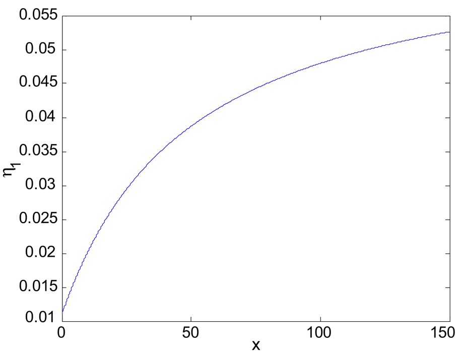
Assume that the positive equilibrium $F_{x y z} (x_{5}^{*}, y_{5}^{*}, z_{5}^{*})$ of system(1)–(3)is locally stable. If $η_{1} (0) > 0$ , then it is globally asymptotically stable (see Fig. 1).

Fig. 1
The plot of the function $η_{1} (x)$ . Here r = 10, K = 150, $α_{1} = 2$ , $α_{2} = 2$ , $a_{1} = 50$ , $a_{2} = 60$ , $d_{1} = 1.3$ , $d_{2} = 0.05$ , $β_{1} = 2$ , $β_{2} = 3$ , δ = 0.2 and γ = 0.007.

The plot of $η_{1} (x)$ indicates that $η_{1} (0) > 0$ for some parameter values. So the assumption $η_{1} (0) > 0$ in Theorem 2.2 makes sense.

Case II

$τ \neq 0$ .

For $τ > 0$ , characteristic equation is given by

λ^{3} + λ^{2} (A + B + C) + λ (A B + B C + C A + D) + A B C + e^{- λ τ} (λ D + E) = 0 .

(13)

Now

λ = i ω

(ω > 0)

in (13) gives

- i ω^{3} - ω^{2} (A + B + C) + i ω (A B + B C + C A + D) + A B C + (\cos ω τ - i \sin ω τ) (i ω D + E) = 0 .

Comparing real and imaginary parts we get,

- ω^{3} + ω (A B + B C + C A) = E \sin ω τ - D ω \cos ω τ,

(14)

- ω^{2} (A + B + C) + A B C = - D ω \sin ω τ - E \cos ω τ .

(15)

Squaring and adding (14) and (15) we get,

ω^{6} + Q_{1} ω^{4} + Q_{2} ω^{2} + Q_{3} = 0,

(16)

where,

\begin{matrix} Q_{1} = A^{2} + B^{2} + C^{2} > 0, \\ Q_{2} = A^{2} B^{2} + B^{2} C^{2} + C^{2} A^{2} - D^{2}, \\ Q_{3} = A^{2} B^{2} C^{2} - E^{2} . \end{matrix}}

(17)

Hence Eq. (16) has unique positive solution

ω_{0}^{2}

, if

Q_{2} > 0

and

Q_{3} < 0

Now, from (14) and (15) we get,

\cos ω τ = [D ω^{4} - D ω^{2} (A B + B C + C A) + E ω^{2} (A + B + C) - E A B C] {[D^{2} ω^{2} + E^{2}]}^{- 1} .

(18)

So, corresponding to

λ = i ω_{0}

, there exists

τ_{0 n}

such that,

τ_{0 n} = \frac{1}{ω_{0}} arc \cos [(D ω_{0}^{4} - ω_{0 n}^{2} {D (A B + B C + C A) - E (A + B + C)} - E A B C) {(D^{2} ω_{0}^{2} + E^{2})}^{- 1}] + \frac{2 n π}{ω_{0}}, n = 0, 1, 2, \dots .

(19)

Now differentiation of (13) with respect to τ gives,

{(\frac{d λ}{d τ})}^{- 1} = [3 λ^{2} + 2 λ (A + B + C) + (A B + B C + C A)] / [λ e^{- λ τ} (λ D + E)] + \frac{D}{λ (λ D + E)} - \frac{τ}{λ} = [3 λ^{3} + 2 λ^{2} (A + B + C) + λ (A B + B C + C A)] / [λ^{2} [e^{- λ τ} (λ D + E)]] + \frac{D}{λ (λ D + E)} - \frac{τ}{λ} = [2 λ^{3} + λ^{2} (A + B + C) - A B C - e^{- λ τ} (λ D + E)] / [λ^{2} e^{- λ τ} (λ D + E)] + \frac{D}{λ (λ D + E)} - \frac{τ}{λ} = [2 λ^{3} + λ^{2} (A + B + C) - A B C] / [- λ^{2} [λ^{3} + λ^{2} (A + B + C) + λ (A B + B C + C A) + A B C]] + \frac{D}{λ (λ D + E)} - \frac{1}{λ^{2}} - \frac{τ}{λ} = [2 λ^{3} + λ^{2} (A + B + C) - A B C] / [- λ^{2} [λ^{3} + λ^{2} (A + B + C) + λ (A B + B C + C A) + A B C]] - \frac{E}{λ^{2} (λ D + E)} - \frac{τ}{λ},

∴ {{(\frac{d λ}{d τ})}^{- 1} |}_{λ = i ω_{0}} = [- 2 i ω_{0}^{3} - ω_{0}^{2} (A + B + C) - A B C] / [ω_{0}^{2} [- i ω_{0}^{3} - ω_{0}^{2} (A + B + C) + i ω_{0} (A B + B C + C A) + A B C]] + \frac{E}{ω_{0}^{2} (D i ω_{0} + E)} - \frac{τ}{i ω_{0}} = \frac{1}{ω_{0}^{2}} [({ω_{0}^{2} (A + B + C) + A B C} + 2 i ω_{0}^{3}) / ({ω_{0}^{2} (A + B + C) - A B C} + i {ω_{0}^{3} - ω_{0} (A B + B C + C A)})] + \frac{E (E - i D ω_{0})}{ω_{0}^{2} (E^{2} + D^{2} ω_{0}^{2})} + i \frac{τ}{ω_{0}} = \frac{1}{ω_{0}^{2}} [[{ω_{0}^{2} (A + B + C) + A B C} + 2 i ω_{0}^{3}] [{ω_{0}^{2} (A + B + C) - A B C} - i {ω_{0}^{3} - ω_{0} (A B + B C + C A)}] / ({ω_{0}^{2} (A + B + c) - A B C}^{2} + {ω_{0}^{3} - ω_{0} (A B + B C + C A)}^{2})] + \frac{E (E - i D ω_{0})}{ω_{0}^{2} (E^{2} + D^{2} ω_{0}^{2})} + i \frac{τ}{ω_{0}},

∴ Re {{| {(\frac{d λ}{d τ})}^{- 1} |}_{τ = i ω_{0}}} = \frac{1}{ω_{0}^{2}} [(ω_{0}^{4} {(A + B + C)}^{2} - A^{2} B^{2} C^{2} + 2 ω_{0}^{6} - 2 ω_{0}^{4} (A B + B C + C A)) / (ω_{0}^{4} {(A + B + C)}^{2} - 2 ω_{0}^{2} A B C (A + B + C) + A^{2} B^{2} C^{2} + ω_{0}^{6} - 2 ω_{0}^{4} (A B + B C + C A) + ω_{0}^{2} {(A B + B C + C A)}^{2})] + \frac{E^{2}}{ω_{0}^{2} (E^{2} + D^{2} ω_{0}^{2})} = \frac{1}{ω_{0}^{2}} [(ω_{0}^{4} (A^{2} + B^{2} + C^{2}) + 2 ω_{0}^{6} - A^{2} B^{2} C^{2}) / (ω_{0}^{6} + ω_{0}^{4} (A^{2} + B^{2} + C^{2}) + ω_{0}^{2} (A^{2} B^{2} + B^{2} C^{2} + C^{2} A^{2}) + A^{2} B^{2} C^{2})] + \frac{E^{2}}{ω_{0}^{2} (E^{2} + D^{2} ω_{0}^{2})} = \frac{1}{ω_{0}^{2}} [\frac{ω_{0}^{4} (A^{2} + B^{2} + C^{2}) + 2 ω_{0}^{6} - A^{2} B^{2} C^{2}}{E^{2} + D^{2} ω_{0}^{2}} + \frac{E^{2}}{E^{2} + D^{2} ω_{0}^{2}}], using (16) = \frac{1}{ω_{0}^{2}} [\frac{ω_{0}^{4} (A^{2} + B^{2} + C^{2}) + 2 ω_{0}^{6}}{E^{2} + D^{2} ω_{0}^{2}} + \frac{E^{2} - A^{2} B^{2} C^{2}}{E^{2} + D^{2} ω_{0}^{2}}] > 0 if A^{2} B^{2} C^{2} < E^{2} i.e. Q_{3} < 0 .

So, we can state the above result as a theorem:

Theorem 2.3

If $F_{x y z}$ exists, $C > 0$ , $Q_{2} > 0$ and $Q_{3} < 0$ , then as τ increases from zero, there is a value $τ_{0}$ such that the interior equilibrium $F_{x y z} (x_{5}^{*}, y_{5}^{*}, z_{5}^{*})$ is locally asymptotically stable when $τ \in [0, τ_{0})$ and unstable when $τ > τ_{0}$ . Further, system (1)–(3) undergoes Hopf-bifurcation at $F_{x y z} (x_{5}^{*}, y_{5}^{*}, z_{5}^{*})$ , when $τ = τ_{0}$ .

Remark 2.1

If the interior equilibrium depends smoothly on a parameter θ in an open interval I of R and if there exists a $θ^{*} \in I$ such that: (i) a simple pair of complex eigenvalues of the variational matrix of the interior equilibrium point exists, say $α (θ) \pm i β (θ)$ such that they become purely imaginary at $θ = θ^{*}$ , whereas the other eigenvalues remain real and negative; and (ii) ${\frac{d α}{d γ} |}_{θ = θ^{*}} \neq 0$ , then at $θ^{*}$ a simple Hopf bifurcation occurs (Liu, [21]). The criterion given by Liu [21] is as follows:

Liu's criterion

If the characteristic equation of the interior equilibrium point is given by

λ^{3} + T_{1} (θ) λ^{2} + T_{2} (θ) λ + T_{3} (θ) = 0,

where

T_{1} (θ)

Δ (θ) = T_{1} (θ) T_{2} (θ) - T_{3} (θ)

T_{3} (θ)

are smooth function of θ in an open interval about

θ^{*} \in R

such that

(I) $T_{1} (θ^{*}) > 0$ , $Δ (θ^{*}) = 0$ , $T_{3} (θ^{*}) > 0$ ,
(II) ${\frac{d Δ}{d θ} |}_{θ = θ^{*}} \neq 0$ , then a simple Hopf bifurcation occurs at $θ = θ^{*}$ .

Now in order to investigate the global stability of $F_{x y z} (x_{5}^{*}, y_{5}^{*}, z_{5}^{*})$ we consider the Lyapunov function

v (x, y, z) = \int_{x_{5}^{*}}^{x} [\frac{β_{1} (\frac{α_{1} η}{a_{1} + η} - \frac{α_{1} x_{5}^{*}}{a_{1} + x_{5}^{*}})}{\frac{α_{1} η}{a_{1} + η}} + \frac{β_{2} (\frac{α_{2} η}{a_{2} + η} - \frac{α_{2} x_{5}^{*}}{a_{2} + x_{5}^{*}})}{\frac{α_{2} η}{a_{2} + η}}] d η + y - y_{5}^{*} - y_{5}^{*} \ln (\frac{y}{y_{5}^{*}}) + z - z_{5}^{*} - z_{5}^{*} \ln (\frac{z}{z_{5}^{*}}) + p \int_{t - τ}^{t} {[x (s) - x_{5}^{*}]}^{2} d s,

where p is some positive constant to be chosen suitably. Now following Theorem 4 of Mukherjee and Roy [16], we arrive at Theorem 2.4 as follows:

Theorem 2.4

Let $K < a_{1}$ , $α_{1} = α_{2}$ , $a_{1} = a_{2}$ and

\frac{γ δ (β_{1} + β_{2})}{{(a_{1} + K)}^{2}} > \frac{K}{2} . \frac{α_{1}^{2}}{r a_{1}^{3}} \frac{{{(β_{1} + β_{2})}^{2} (γ + δ) + δ β_{1}^{2} + γ β_{2}^{2}}}{a_{1} - K},

then the interior equilibrium of system (1)–(3) is globally asymptotically stable.

3 Simulation and discussion

In this article we have studied the dynamical behaviors of a two predator one prey system. The interaction between prey and predators are assumed to be governed by a Holling type II functional response. Here two predators are competing for a single prey.

Often we come across several biological systems in nature exhibiting cyclical behavior. Due to this cyclic nature some populations exhibit periodic fluctuation in abundance, with periodic crashes. One could avoid such crashes and stabilize the population by controlling one of the interacting species (Hudson et al. [22]). Thus it is relevant to find conditions under which a multispecies system exhibits cyclic behavior, and it is equally important to find conditions under which cycles can be prevented in a multispecies system.

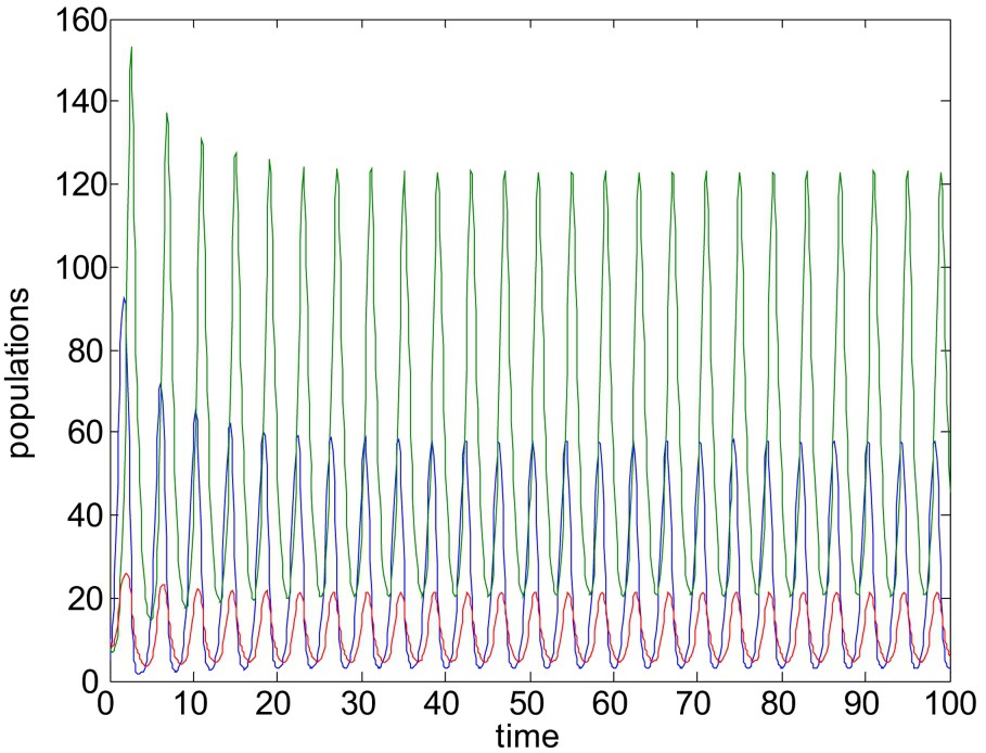
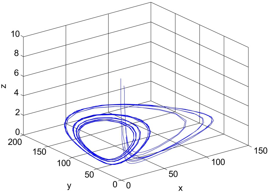
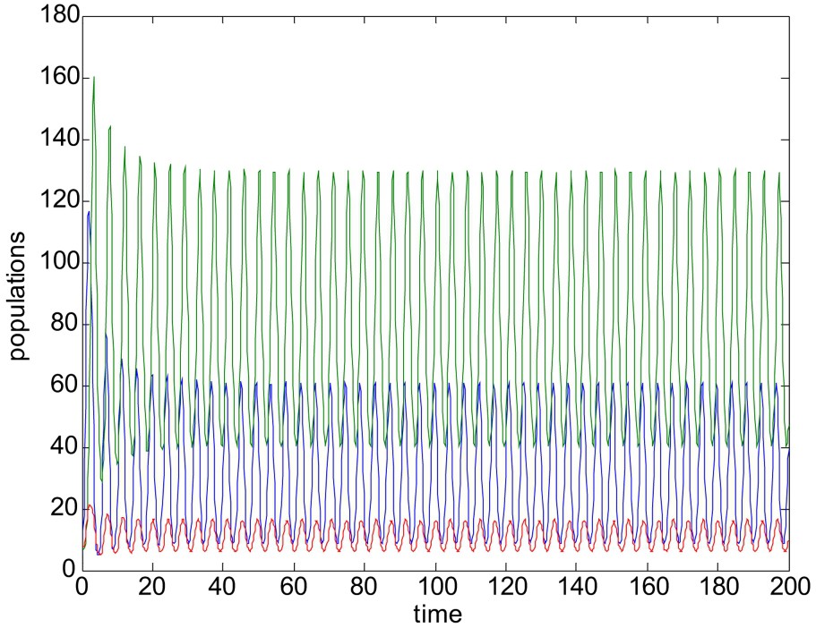
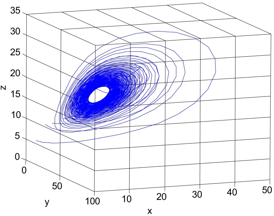
First we consider the case with $τ = 0$ . To illustrate the analytical results numerically, let us take $r = 3.5$ , $K = 150$ , $α_{1} = 2$ , $α_{2} = 2$ , $a_{1} = 35$ , $a_{2} = 45$ , $d_{1} = 1.3$ , $d_{2} = 0.05$ , $β_{1} = 2$ , $β_{2} = 3$ , $δ = 0.2$ . For these values of parameters a super critical Hopf-bifurcation occurs when $γ^{*} = 0.00608308$ . Now if we gradually increase the value of γ, keeping other parameters fixed, then $F_{x y z}$ achieves stability from instability as γ crosses its critical value $γ^{*} = 0.00608308$ (see Figs. 2, 3 and 4).

Fig. 2
Unstable solution of system (1)–(3). Here parameter values are r = 3.5, K = 150, $α_{1} = 2$ , $α_{2} = 2$ , $a_{1} = 35$ , $a_{2} = 45$ , $d_{1} = 1.3$ , $d_{2} = 0.05$ , $β_{1} = 2$ , $β_{2} = 3$ , δ = 0.2, $γ (= 0.005) < γ^{*}$ .

Fig. 3
When $γ = 0.007 > γ^{*}$ , clearly the populations approach to their equilibrium values in finite time. Here parameter values are r = 3.5, K = 150, $α_{1} = 2$ , $α_{2} = 2$ , $a_{1} = 35$ , $a_{2} = 45$ , $d_{1} = 1.3$ , $d_{2} = 0.05$ , $β_{1} = 2$ , $β_{2} = 3$ , δ = 0.2.

Fig. 4
For $γ = γ^{*}$ , there is a limit cycle near $F_{x y z}$ .

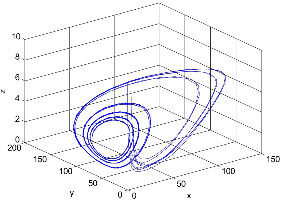
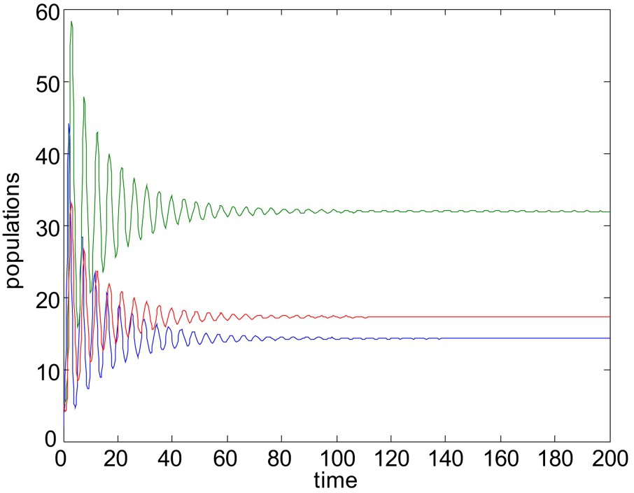
Next consider $α_{1}$ (the maximum value of the per capita reduction rate of x due to y) as the bifurcation parameter. With parameter values $r = 3.5$ , $K = 150$ , $a_{1} = 35$ , $α_{2} = 2$ , $a_{2} = 45$ , $d_{1} = 1.3$ , $b_{1} = 2$ , $γ = 0.006$ , $d_{2} = 0.05$ , $b_{2} = 4$ , $δ = 0.2$ , a Hopf-bifurcation occurs when $α_{1}^{*} = 2.071026$ (see Figs. 5, 6, and 7).

Fig. 5
When $α_{1} = 1.9 < α_{1}^{*}$ , clearly the populations approach to their equilibrium values in finite time. Here parameter values are r = 3.5, K = 150, $a_{1} = 35$ , $α_{2} = 2$ , $a_{2} = 45$ , $d_{1} = 1.3$ , $b_{1} = 2$ , γ = 0.006, $d_{2} = 0.05$ , $b_{2} = 4$ , δ = 0.2.

Fig. 6
Unstable solution of system (1)–(3). Here all the parameters are same as in Fig. 5, except $α_{1} = 2.5 > α_{1}^{*}$ .

Fig. 7
For $α_{1} = α_{1}^{*}$ , there is a limit cycle near $F_{x y z}$ .

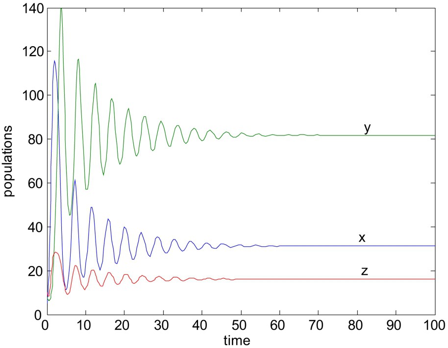
The numerical study presented here shows that, using parameter γ or $α_{1}$ as control, it is possible to break unstable behavior of the system (1)–(3) and drive it to a stable state. Also it is possible to keep the population levels at a required state using the above control.

Now we would like to mention that the stability criteria of the system without delay do not necessarily guarantee the stability of the system with delay. It has been shown that the positive equilibrium which is stable without delay, remains stable under certain conditions when the time delay is less than the threshold value, otherwise the stable equilibrium become unstable. To illustrate the results numerically, choose $r = 2.5$ , $K = 100$ , $α_{1} = 2$ , $α_{2} = 2$ , $a_{1} = 30$ , $a_{2} = 35$ , $d_{1} = 0.03$ , $d_{2} = 0.02$ , $b_{1} = 5$ , $b_{2} = 6$ , $γ = 0.1$ , $δ = 0.2$ (Figs. 8 and 9).

Fig. 8
When $τ = 0.65 < τ_{0}$ , clearly the populations approach to their equilibrium values in finite time.

Fig. 9
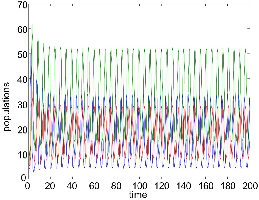
Unstable solution of system (1)–(3). Here all the parameters are same as in Fig. 8, except $τ = 0.79 > τ_{0}$ .

For the above choices of parameters $F_{x y z} (x_{5}^{*}, y_{5}^{*}, z_{5}^{*})$ is locally asymptotically stable in the absence of delay. Now for the same values of parameters, it is seen from the Theorem 2.3, that there exists a critical value of $τ = τ_{0} = 0.711633041$ and $F_{x y z}$ losses its stability as τ crosses the critical value $τ_{0}$ (Fig. 10).

Fig. 10
For $τ = τ_{0} = 0.711633041$ , there is a limit cycle near $F_{x y z}$ .

We have also given some graphical support in favor of our numerical results.