Analysis of population structure and genetic diversity of Egyptian and exotic rice (<i>Oryza sativa</i> L.) genotypes

Khaled F.M. Salem; Ahmed Sallam

doi:10.1016/j.crvi.2015.11.003

Genetics / Génétique

Analysis of population structure and genetic diversity of Egyptian and exotic rice (Oryza sativa L.) genotypes

Khaled F.M. Salem ¹; Ahmed Sallam ^2,³

¹ Plant Biotechnology Department, Genetic Engineering and Biotechnology Research Institute (GEBRI), University of Sadat City, P. O. Box 79, Sadat City, Egypt
² Department of Genetics, Faculty of Agriculture, Assiut Univeristy, Assiut 71526, Egypt
³ Department of Agronomy & Horticulture, University of Nebraska-Lincoln, NE 68683-0915, USA

Comptes Rendus. Biologies, Volume 339 (2016) no. 1, pp. 1-9.

Abstract

Understanding the population structure and genetic diversity is a very important goal to improve the economic value of crops. In rice, a loss of genetic diversity in the last few centuries is observed. To address this challenge, a set of 22 lines from three different regions – India (two), and Philippines (six), and Egypt (14) – were used to assess the genetic diversity and the features of population structure. These genotypes were analyzed using 106 SSR alleles that showed a clear polymorphism among the lines. Genetic diversity was estimated based on the number of different alleles, polymorphism information content (PIC), and gene diversity. A total of 106 SSR alleles was identified from the 23 SSR loci and used to study the population structure and carry out a cluster analysis. All SSR loci showed a wide range of the number of different alleles extended from two (one loci) to seven alleles (three loci). Five and eight loci showed high PIC and gene diversity (≥ 0.70), respectively. The results of population structure are in agreement with cluster analysis results. Both analyses revealed two different subpopulations (G1 and G2) with different genetic properties in number of private alleles, number of different alleles (Na), number of effective alleles (Ne), expected heterozygosity (He), and Shannon's Information Index (SII). Our findings indicate that five SSR loci (RM 111, RM 307, RM 22, RM 19, and RM 271) could be used in breeding programs to enhance the marker-assisted selection through QTL mapping and association studies. A high genetic diversity found between genotypes which can be exploited to improve and produce rice cultivars for important traits (e.g. high agronomic features and tolerance to biotic or/and abiotic stresses).

Metadata

Received: 2015-09-28
Accepted: 2015-11-16
Published online: 2015-12-23

PMID

DOI: 10.1016/j.crvi.2015.11.003

Keywords: Rice, Genetic diversity, Population structure, SSR

Author's affiliations:

Khaled F.M. Salem ¹; Ahmed Sallam ^{2, 3}

¹ Plant Biotechnology Department, Genetic Engineering and Biotechnology Research Institute (GEBRI), University of Sadat City, P. O. Box 79, Sadat City, Egypt
² Department of Genetics, Faculty of Agriculture, Assiut Univeristy, Assiut 71526, Egypt
³ Department of Agronomy & Horticulture, University of Nebraska-Lincoln, NE 68683-0915, USA

@article{CRBIOL_2016__339_1_1_0,
     author = {Khaled F.M. Salem and Ahmed Sallam},
     title = {Analysis of population structure and genetic diversity of {Egyptian} and exotic rice {(\protect\emph{Oryza} sativa} {L.)} genotypes},
     journal = {Comptes Rendus. Biologies},
     pages = {1--9},
     publisher = {Elsevier},
     volume = {339},
     number = {1},
     year = {2016},
     doi = {10.1016/j.crvi.2015.11.003},
     language = {en},
}

TY  - JOUR
AU  - Khaled F.M. Salem
AU  - Ahmed Sallam
TI  - Analysis of population structure and genetic diversity of Egyptian and exotic rice (Oryza sativa L.) genotypes
JO  - Comptes Rendus. Biologies
PY  - 2016
SP  - 1
EP  - 9
VL  - 339
IS  - 1
PB  - Elsevier
DO  - 10.1016/j.crvi.2015.11.003
LA  - en
ID  - CRBIOL_2016__339_1_1_0
ER  -

%0 Journal Article
%A Khaled F.M. Salem
%A Ahmed Sallam
%T Analysis of population structure and genetic diversity of Egyptian and exotic rice (Oryza sativa L.) genotypes
%J Comptes Rendus. Biologies
%D 2016
%P 1-9
%V 339
%N 1
%I Elsevier
%R 10.1016/j.crvi.2015.11.003
%G en
%F CRBIOL_2016__339_1_1_0

Khaled F.M. Salem; Ahmed Sallam. Analysis of population structure and genetic diversity of Egyptian and exotic rice (Oryza sativa L.) genotypes. Comptes Rendus. Biologies, Volume 339 (2016) no. 1, pp. 1-9. doi : 10.1016/j.crvi.2015.11.003. https://comptes-rendus.academie-sciences.fr/biologies/articles/10.1016/j.crvi.2015.11.003/

Original version of the full text

The full text below may contain a few conversion errors compared to the version of record of the published article.

1 Introduction

Rice is considered one of the most important cultivated crops because it supplies food for one-half of the world-human populations and occupies the second rank for consumption after wheat [1]. Egypt is ranked 15 with 4,600,000 tons among the countries with the highest rice production, and is the biggest producer in the Near East region (world rice production, 2015). More attention is paid to the production of rice in the lower bay of the Nile River. However, due to limited water resources, rice cultivation has been limited in Egypt. Moreover, a dramatic loss of diversity in rice has been observed in the last centuries [2]. Therefore, producing new rice cultivars is urgently needed, not only to meet the demand of world population, but also to overcome such problems of abiotic and biotic stresses.

The increase in the production and in the ability to resist the abiotic stresses can be achieved through a crop improvement effort [3]. This depends on the availability of genetic diversity existing in the rice cultivars that could be integrated in breeding programs. Thus, studying and quantifying the genetic variation among different genetic backgrounds is considered a vital goal to expand the diversity among cultivars. This diversity can be useful for producing high-yield cultivars in combination with resistance to abiotic stresses such as drought and salt, which are the most important abiotic stresses in Egypt (FAO, 2004). Two ways can be used to address the genetic variability:

• based on morphological traits;
• based on differences in the DNA detected by DNA molecular markers.

Assessing genetic diversity based on morphological traits have some shortcomings, including the influence by the environmental factors, the lack of resolution power that is required for discriminating between very closely genotypes, and time consuming since many locations and years should be investigated to achieve the goal [4]. On the other hand, the development of molecular DNA markers results in significant advances in the evaluation of the genetic diversity in many crop species [4].

Among these DNA markers, single sequence repeats (SSR) provide a high level of polymorphism that can be utilized to study diversity between species [5]. Thus, SSR markers are very useful and had been used before to study genetic diversity in rice [2,6,7]. Genetic diversity in earlier studies was described using cluster analysis to figure out the relatedness between genotypes. Advances in population structure have led to the development of many pieces of software that provide a better understanding of the genetic structure of the population. Among these pieces of software, STRUCTURE produces meaningful clusters based on Hardy–Weinber disequilibrium and linkage disequilibrium (LD) caused by admixture between populations [8]. Taking into account the LD between individuals improves clustering results [9]. This leads to fruitful usefulness of the genetic diversity that can be used in breeding programs to produce new cultivars carrying genes for increasing the yield and the resistance to abiotic stresses.

The objectives of this study are:

• to assess the population structure in the elite 22 selected rice lines;
• to assess the mount of genetic diversity among them using SSR markers;
• to compare the genetic properties among subpopulation.

2 Material and methods

2.1 Plant materials

In total, a diverse collection of 22 Egyptian and exotic rice (Oryza sativa L.) genotypes (India and Philippines) were randomly selected and used in this study. The genotypes were supplied by the Agricultural Research Center (ARC, Giza, Egypt), the International Rice Research Institute, (Los Banos, Philippines), and the National Small Grain Collection (USDA, ARS, USA). A list of the used rice genotypes together with details are presented in Table 1.

Number of genotype	Genotype Name	Origin	Subspecies Group
1	IR 20	Philippines	Indica
2	IR 22	Philippines	Indica
3	IR 24	Philippines	Indica
4	IR 50	Philippines	Indica
5	IR 64	Philippines	Indica
6	IR 74	Philippines	Indica
7	Bala	India	Indica
8	IET 1444	India	Indica
9	Arabi	Egypt	Japonica
10	Agamy M1	Egypt	Japonica
11	Nahda	Egypt	Japonica
12	Yabani M1	Egypt	Japonica
13	Yabani M7	Egypt	Japonica
14	Yabani 15	Egypt	Japonica
15	Yabani lulu	Egypt	Japonica
16	Giza 14	Egypt	Japonica
17	Giza 171	Egypt	Japonica
18	Giza 172	Egypt	Japonica
19	Giza 177	Egypt	Japonica
20	Giza 178	Egypt	Indica/Japonica
21	Giza 181	Egypt	Indica
22	Gz 1386-5-4	Egypt	Indica

2.2 DNA isolation

Total genomic DNA was extracted from fresh seedling leaves for each genotype. Young leaves from eight-week-old rice plants were cut as tissue samples for DNA extraction. DNA was isolated from these genotypes as described by McCouch et al. [10].

2.3 Microsatellite markers analysis

In total, twenty-three rice microsatellite markers for 23 loci representing at least one microsatellite marker from chromosomes (1, 2, 3, 4, 5, 6, 7, 8, 9, 10, 11 and 12) (Table 2) were selected for genotyping the rice lines [11,12]. All Rice Microsatellites (RM) used were dinucleotide repeats, whereas RM552, RM144, RM19 and RM307 had a trinucleotide or complex motif. Microsatellite amplifications, polymerase chain reaction and fragment analysis were carried out as reported by [11] and [12]. Table 2 shows the fragment detection for SSR markers used in this study. RM designation, chromosomal location, motif, annealing temperature (C), repeat category and expected fragment size (bp) of the amplified loci were reported by [11] and [12].

Number	SSR primers	Chromosomal location	Motif	Annealing temperature (T_m, °C)	Repeat category	Expected fragment size (bp)
1	RM 5	1	(GA)14	55	di	84
2	RM151	1	(TA)23	55	di	197
3	RM6	2	(AG)16	55	di	163
4	RM154	2	(GA)21	60	di	106
5	RM22	3	(GA)22	55	–	194
6	RM55	3	(GA)17	55	di	213
7	RM307	4	(AT)14(GT)21	55	Complex	104
8	RM161	5	(AG)20	60	di	116
9	RM 413	5	(AG)11	50	di	65
10	RM133	6	(CT)8	60	di	224
11	RM162	6	(AC)20	60	di	130
12	RM11	7	(GA)17	55	di	115
13	RM118	7	(GA)8	60	di	106
14	RM408	8	(CT)13	55	di	109
15	RM433	8	(AG)13	50	di	215
16	RM215	9	(CT)16	55	di	126
17	RM285	9	(GA)12	55	–	205
18	RM271	10	(GA)15	55	di	65
19	RM 474	10	(AT)13	55	di	195
20	RM552	11	(TAT)13	55	tri	153
21	RM144	11	(ATT)11	55	tri	208
22	RM19	12	(ATC)10	55	tri	195
23	RM277	12	(GA)11	55	di	108

2.4 Genetic diversity and AMOVA

The summary statistics of the marker data such as gene diversity, and polymorphism information content (PIC) were calculated using PowerMarker software V 3.25 [13]. The PIC value as a relative value for each marker according to the amount of existing polymorphism was described by [14].

The value of PICs was calculated using the following formula:

{PIC}_{i} = 1 - \sum_{j = 1}^{n} P_{i j}^{2} - \sum_{j = 1}^{n - 1} \sum_{k = j + 1}^{n} 2 P_{i j}^{2} P_{i k}^{2}

where P_ij and P_ik are the frequencies of the jth and kth alleles for marker i. The gene diversity is calculated as the probability that two alleles randomly selected from the test sample be different. The common biased estimator of the gene diversity for marker i can be estimated using the aforementioned equation by dropping the last part as fully described in [15] and [16].

Analysis of molecular variance (AMOVA) with 1000 permutations, number of different alleles, effective number of alleles, the expected heterozygosity, and Shannon's Information Index (SII) were performed using GeneAlEx 6.41 [17].

2.5 Population structure and clustering

The population structure (PS) was used to reveal whether or not there are subgroups. The PS implied using the Bayesian model-based software program STRUCTURE 2.2 [8]. In this analysis, the SSR markers were converted to 1 vs. 0 in order to cover all possible polymorphisms. As a result, a number of 106 SSR alleles were obtained and used in the analysis. The program was set on 100,000 as burn-in iteration, followed by 100,000 Markov chain Monte Carlo (MCMC) replications after burn-in. The admixture and allele frequencies correlated models were selected. The population structure analysis was run with five independent iterations. The number of subpopulations (k) ranged from 1 to 10. The estimated likelihood value of data [lnP(D)] from the STRUCTURE output was plotted against the ad hoc statistics Δk. The best k value was determined according to Evanno et al. [18]. The change rate in the log probability of data between k values that best demonstrates the population structure-based on maximizing log probability or the value at which LnP(D) reaches a plateau was illustrated using Microsoft Excel 2010.

The cluster analysis of all genotypes was done using Jaccard's dissimilarity index as a proximity matrix, as described by Jaccard in 1908. A neighbor-joining (NJ) relationship using parsimony substitution models and an unweighted pair group method with arithmetic mean (UPGMA) was carried out using R software package. All graphical analyses were done using Microsoft Office Excel 2010.

3 Results

The PIC, gene diversity, and number of different alleles per locus are presented on Fig. 1. The 23 SSR loci were used to determine the genetic diversity. The gene diversity and PIC averaged 0.62 and 0.57, with ranges of 0.38–0.79 and 0.34 and 0.76 (Fig. 1a). The RM271 locus showed the highest PIC and gene diversity among all SSR loci. The number of different alleles per locus extended from two for marker RM161 to seven for markers RM144, 307, and 474 (Fig. 1b). The major allele frequency had an average of 0.50 with a range extended from 0.27 to 0.72 (data not shown).

Fig. 1
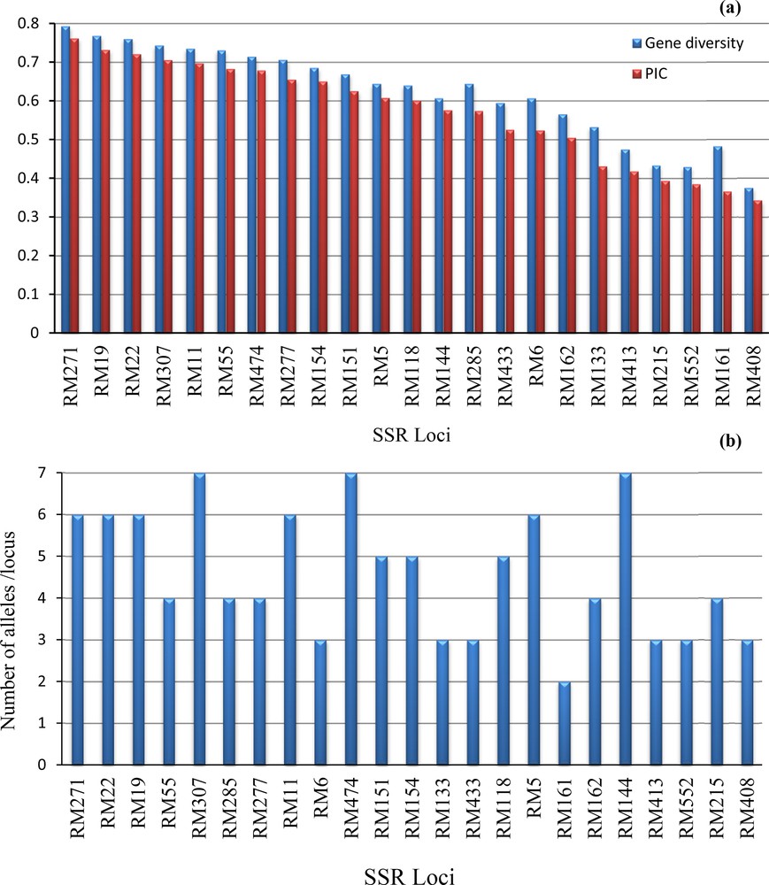
Distribution of genetic diversity of 106 SSR markers used in the genetic diversity analysis 22 rice genotypes. (a). Gene diversity and Polymorphic Information Content (PIC) for each marker, and (b) number of different alleles per loci.

A total of 106 alleles were detected from a set of 23 SSR loci on a panel of 22 rice genotypes. STRUCTURE analysis software was used to study the population structure (i.e. genetic relatedness) and determine the subpopulations (k) of the 22 rice genotypes based on the distribution of the 106 SSR alleles evaluated in this study. The best number of subpopulations was determined by plotting the number k against the calculated likelihood value [lnP(D)] obtained from STRUCTURE runs. Obviously, lnP(D) showed to be an increasing function of k for all the values observed (Fig. 2a). Structure simulation described that the calculated average of lnP(D) against k = 2 was addressed to be the best k, indicating that two subpopulations could include all the 22 rice genotypes with the highest probability. This can be also confirmed by plotting the number k against Δk. A sharp peak was found for k = 2 (Fig. 2b). Therefore, a k value of two was chosen to demonstrate the genetic structure of the 22 rice genotypes (Fig. 3). The estimated population structure suggested that genotypes with partial membership exhibited distinctive identities (e.g., Bala and Yabani_M1).

Fig. 2
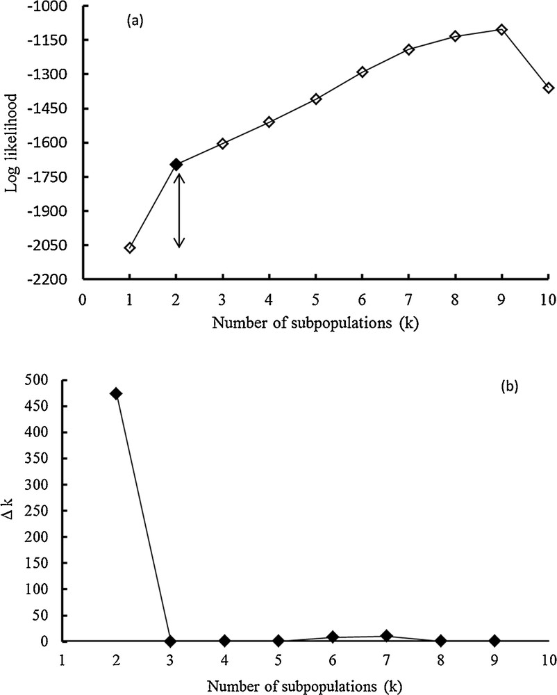
Population structure analysis of rice genotypes using 106 SSRs; (a) shows the average log–likelihood value (using STRUCTURE), (b) shows ΔK for differing numbers of subpopulations (k). Within the population (using STRUCTURE). Unfilled square point refer to the best k = 2.

Fig. 3
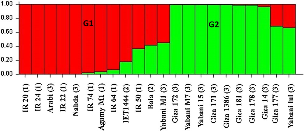
Estimated population structure of 20 rice genotypes (k = 2). The y-axis corresponds to the subgroup membership, and the x-axis to the genotype. G (G1and G2). Stands for a subpopulation. The genotypes from the Philippines are marked by (1), from India by (2), and from Egypt by (3).

A significant divergence was found among subpopulations and average distance (expected heterozygosity) among genotypes in the same subpopulations (Table 3). Subpopulation 1 (G1) included genotypes from different parts: Egypt, India, and the Philippines, while all genotypes in subpopulation 2 (G2) were from Egypt. In our cluster analysis, two subclusters can be distinguished (Fig. 4): C1 and C2. C1 included 12 genotypes: six genotypes from the Philippines (IR 20, IR 22, IR 24, IR 50, IR 64, and IR 74), four genotypes from Egypt (Arabi, Agamy, M1 Nahda, and Yabani M1), and two genotypes from India (Bala and IET 1444). C2 included the other 10 genotypes from Egypt (Yabani M7, Yabani 15, Yabani lulu, Giza 14, Giza 171, Giza 172, Giza 177, Giza 178, Giza 181, and Gz 1386-5-4). The genetic distance between genotypes in C1 ranged from 0.75 to 0.86, while it ranged from 0.48 to 0.90 in C2. Noticeably, four Egyptian genotypes were grouped and cluster with Indian and Philippian genotypes. Interestingly, the genotypes in each subgroup (G1 and G2) detected by STRUCTURE were the same genotypes identified using the Jaccard and UPGMA (C1 and C2) distance-based methods. Within and among two subpopulation groups of rice genotypes, the components of the total genetic variation were estimated by AMOVA (Table 4). The analysis showed that the within-population diversity explained most of the genetic diversity (74%) when compared to among-population diversity (26%).

Subpopulation groups	F _ST	Heterozygosity	Number of genotypes
G1	0.4645	0.2008	6 (Philippines), 4 (Egypt), 2 (India)
G2	0.3429	0.2373	10 (Egypt)

Fig. 4
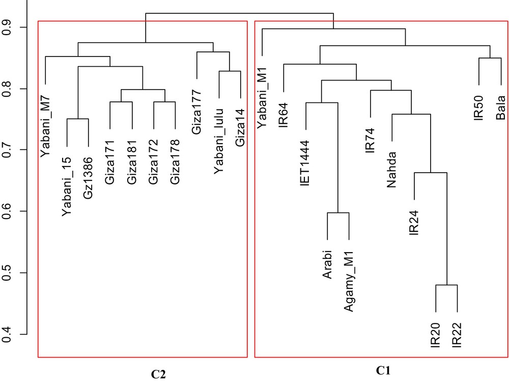
Cluster analysis (C) based on the genetic distance for the 20 rice genotypes.

Source of variation	df	SS	MS	Est. Var.	%	P value
Among subpopulations	1	122.861	122.861	8.916	26	0.001
Within subpopulation	20	511.867	25.593	25.593	74	0.001
Total	21	634.727		34.510	100	0.001

The number of loci with a private allele for each genotype in both subpopulations is presented in Fig. 5a and b. The G1 contained the highest number of loci with private alleles (102) than in G2 (70). In G1, the number of loci with private alleles ranged from 7 (IR 20) to 10 (IR24) with an average of 8.5 per locus. The number of loci with private alleles in G2, on the other hand, ranged also from 7 (Giza 172 and Yabani_lulu) to 10 (Yabani_M7), with an average of seven per locus.

Fig. 5
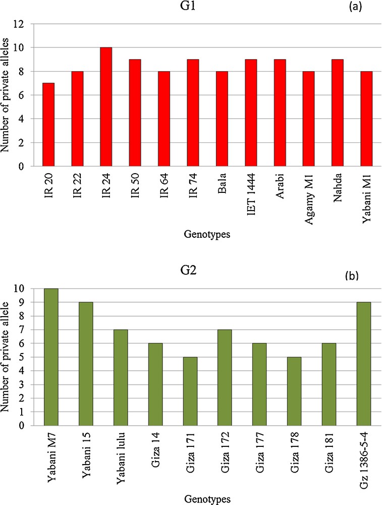
Distribution of private alleles in each population: (a) population 1 (G1) and (b) population 2 (G2).

Table 5 shows the allelic pattern for each locus across two subpopulations. The highest number of different alleles (Na) in both populations was five. Of these five, two markers (RM474 and RM19) were found in both populations. The lowest Na in G1 was found in seven loci with two alleles and two loci with one allele in G2. The number of effective alleles ranged from 1.18 (RM552, 151, 154, and 161) to 3.60 (RM5) in G1 and from 1 (RM162 and 433) to 4.54 (RM22). All loci in both subpopulations did not show any heterozygosity. The expected heterozygosity was calculated for each locus in both populations. The highest expected heterozygosity in G1 was found for RM5 (0.72) and for RM22 (0.78) in G2. Of those loci in G2, two loci (RM162 and 433) showed also zero expected heterozygosity. Shannon's Information Index (SII) ranged from 0.29 (RM151, 154, 161, and 552) to 1.42 (RM5) in G1, while it extended from 0 (RM162 and 433) to 1.52 (RM22). On average, both populations showed approximately an equal number of different and private alleles. The number of effective alleles was higher in G2 (2.412) than in G1 (2.232). G2 showed a higher expected heterozygosity than G1. The polymorphic locus in G1 was 100%, while it was 91% in G2.

Loci	Population 1 (G1)	Population 2 (G2)
	N_a	N_e	H_e	SII	N_a	N_e	H_e	SII
RM5	5.00	3.60	0.72	1.42	4.00	1.92	0.48	0.94
RM6	2.00	1.80	0.44	0.64	3.00	2.63	0.62	1.03
RM11	5.00	2.57	0.61	1.23	3.00	2.78	0.64	1.06
RM22	4.00	3.13	0.68	1.24	5.00	4.55	0.78	1.56
RM133	2.00	2.00	0.50	0.69	3.00	2.17	0.54	0.90
RM215	2.00	1.38	0.28	0.45	4.00	2.38	0.58	1.09
RM271	4.00	2.88	0.65	1.20	2.00	2.00	0.50	0.69
RM277	3.00	3.00	0.67	1.10	3.00	2.63	0.62	1.03
RM307	4.00	1.71	0.42	0.84	4.00	2.94	0.66	1.22
RM413	2.00	1.95	0.49	0.68	2.00	1.47	0.32	0.50
RM552	2.00	1.18	0.15	0.29	3.00	2.63	0.62	1.03
RM55	4.00	2.40	0.58	1.08	4.00	3.33	0.70	1.28
RM118	3.00	2.88	0.65	1.08	3.00	1.85	0.46	0.80
RM144	4.00	2.67	0.63	1.13	5.00	2.50	0.60	1.23
RM151	2.00	1.18	0.15	0.29	3.00	2.63	0.62	1.03
RM154	2.00	1.18	0.15	0.29	4.00	3.57	0.72	1.31
RM161	2.00	1.18	0.15	0.29	2.00	1.47	0.32	0.50
RM162	4.00	2.88	0.65	1.20	1.00	1.00	0.00	0.00
RM285	4.00	2.48	0.60	1.11	3.00	1.85	0.46	0.80
RM433	3.00	2.57	0.61	1.01	1.00	1.00	0.00	0.00
RM474	5.00	2.12	0.53	1.20	5.00	3.57	0.72	1.42
RM19	5.00	3.00	0.67	1.31	5.00	3.13	0.68	1.36
RM408	2.00	1.60	0.38	0.56	2.00	1.47	0.32	0.50
Mean	3.26	2.23	0.49	0.88	3.22	2.41	0.52	0.92
SE	0.25	0.15	0.04	0.07	0.25	0.18	0.04	0.08

4 Discussion

The PIC values of the 22 SSR loci showing high values extend from 0.34 to 0.76 (Fig. 1a), with an average of 0.57. This average indicates higher genetic diversity among the rice genotypes selected in this study. PIC presents the informativeness of SSR loci and their features to detect differences among genotypes [1]. Of the 22 SSR loci, five (RM19, 11, 22, 271, and 307) showed very high PIC values (0.70 < PIC > 0.76). These high SSR loci can be used to expand the genetic basis of the current genotypes. Similar average PIC values were reported by some authors [3,19–22]. Basically, there are many factors that affect PIC values, including the breeding mode of the species, the genetic diversity in the selected genotypes, the population size, the genotypic method, and locations of primers in the genome used for the study [23]. High gene diversity was found in the current genotypes ranging from 0.37 to 0.79, with an average of 0.62. This result is in close agreement with the finding reported by [3] in 82 rice genotypes. The SSR loci showed a high variation of the number of different alleles that ranged from 2 for RM161 to 7 alleles for three loci (RM144, 307, and 474), with an average of 4.5 alleles per locus. Similar results were obtained by [24]. Of the 23 loci, the number of different alleles of 11 SSR loci (RM5, 55,118, 133, 154, 215, 271, 277, 413, 433, and 474) was reported by [1] in a set of 82 rice genotypes. Three loci (RM133, 154, and 271) showed the same number of different alleles in the present study and [3]. A high significant correlation was found between the number of alleles and both PIC (r = 0.71**) and gene diversity (r = 0.78**). This indicates a further explanation for the high genetic diversity found among the 22 rice genotypes. These SSR loci are highly fruitful and can be used for genetic diversity studies.

In this study, 106 SSR alleles, obtained from the 23 SSR loci, were used to estimate the population structure of 22 rice genotypes from three parts: Egypt, India, and Philippines. SSRs have been established in previous studies as DNA markers that show a high level of polymorphism in plants [25]. The 22 rice genotypes were grouped into two subpopulations with significant divergence among subpopulations (P > 0.001). Similar findings were reported by [23]. The analysis of AMOVA revealed a high genetic diversity within populations (74%). The genetic diversity among subpopulation was low, with 26%. This low genetic differentiation among genotypes may be due to gene flow that resulted from the movement of seeds [26]. Farmers tend to exchange seeds in order to maximize the diversity of local germplasms. This leads to an increase in the distribution of alleles among different populations regardless of their geographical distance [27]. A high genetic diversity among populations (92.12%) and a very low genetic diversity within populations (7.88%) were reported by [2] in five rice populations. On the other hand, the genetic diversity was distributed with 4% among populations (12 populations), 70% among individual, 25% within individual, and 1% among region for 375 rice genotypes [23]. The high level of polymorphism found among the genotypes in G1 (100%) and G2 (91%) can be exploited in breeding programs to maximize the genetic diversity [24].

The results of UPGMA cluster analysis was in agreement with population structure. All the 22 genotypes were clustered to two groups with the same genotypes as revealed by STRUCTURE. Genetic distance (Fig. 4) ranged from 0.48 to 0.90, indicating the magnitude of the genetic diversity among the elite genotypes. Obviously, the C1 (cluster 1) that represented population 1 (G1) showed higher genetic diversity than C2. This is not surprising, since C1 included 12 genotypes covering three different regions (Egypt, India, and Philippines), while G2 (or C2) showed low genetic diversity because it contained genotypes from one region (Egypt).

The two populations showed an observable variation in loci carrying private alleles (Fig. 5a and b). On average, G1 carried a higher number of loci with private alleles than G2, indicating the existence of a high genetic diversity among G1 genotypes. The private alleles provide a unique genetic variability in certain loci. Moreover, the information gained from the presence of private alleles is quite fruitful to identify high-diverse genotypes that can be integrated in breeding programs as parents to increase the allele richness in the gene banks [28,29].

Each population showed a specific allelic pattern (Table 5). The SSR loci in both populations showed a very slight difference in the range of the different alleles (Na) and the effective alleles (Ne). No heterozygosity was observed in any SSR locus due the highly homozygosity of the genotypes. Moreover, rice is a self-pollinated crop and hence SSR markers should indicate only one allele per locus. Therefore, the observed heterozygosity should be zero. However, the range of the expected heterozygosity was higher in G1 (0.15–0.72) than in G2 (0–0.78). The expected heterozygosity (He) of loci describes very important information for genetic variability in population genetics [30]. All SSR loci in G1 presented Shannon's Information Indices (SII) within a range of 0.19–1.42. Of the 23 SSR loci, two (RM162 AND RM433) showed no SII in G2. This indicates all loci are informative in the G1 due to its diverse genotypes. High positive correlations were found between SII and Ne in both G1 (r = 0.89**) and G2 (0.93**).

The G1 provides a useful source of genetic diversity in rice because it included genotypes from three different parts (Egypt, India, and Philippines). These genotypes can be used in future breeding programs to maximize the genetic diversity in rice. Such diversity could be very useful in marker-assisted selection and genome-wide association studies by creating multi-parent advanced generation inter-cross (MAGIC).

5 Conclusion

The result of this work demonstrates the advantages of SSR markers for studying the genetic diversity among rice genotypes. Studying the genetic diversity among individuals within populations is very useful in selecting the genotypes as candidate parents in future breeding programs to improve the target traits in rice. Furthermore, it is recommendable to understand the allele pattern in subpopulations, since it sheds light on the informative loci that can be effectively used to study genetic diversity.

Disclosure of interest

The authors declare that they have no competing interest.

References

[1] J. Maclean; B. Hardy; G. Hettel Rice almanac, International Rice Research Institute, 2013 http://irri.org/resources/publications/books/rice-almanac-4th-edition

[2] G. Choudhary; N. Ranjitkumar; M. Surapaneni; D.A. Deborah; A. Vipparla; G. Anuradha et al. Molecular genetic diversity of major Indian rice cultivars over decadal periods, PLoS One, Volume 8 (2013), p. e66197 | DOI

[3] B.K. Babu; V. Meena; V. Agarwal; P.K. Agrawal Population structure and genetic diversity analysis of Indian and exotic rice (Oryza sativa L.) accessions using SSR markers, Mol. Biol. Rep., Volume 41 (2014), pp. 4329-4339 | DOI

[4] R. Cooke Variety identification of crop plants (J.H. Skerrit; R. Appels, eds.), New Diagnostics in Crop Science. Biotechnology in Agriculture, 13, CAB International, Wallingford, UK, 1995, pp. 33-63

[5] J.S.C. Smith; E.C.L. Chin; H. Shu; O.S. Smith; S.J. Wall; M.L. Senior et al. An evaluation of the utility of SSR loci as molecular markers in maize (Zea mays L.): comparisons with data from RFLPS and pedigree, Theor. Appl. Genet., Volume 95 (1997), pp. 163-173 | DOI

[6] H.A. Agrama; G.C. Eizenga; W. Yan Association mapping of yield and its components in rice cultivars, Mol. Breed., Volume 19 (2007), pp. 341-356 | DOI

[7] T.C. de Oliveira Borba; R.P.V. Brondani; F. Breseghello; A.S.G. Coelho; J.A. Mendonça; P.H.N. Rangel et al. Association mapping for yield and grain quality traits in rice (Oryza sativa L.), 33 (2010), pp. 515-524 | DOI

[8] J.K. Pritchard; M. Stephens; P. Donnelly Inference of population structure using multilocus genotype data, Genetics, Volume 155 (2000), pp. 945-959 http://www.pubmedcentral.nih.gov/articlerender.fcgi?artid=1461096&tool=pmcentrez&rendertype=abstract (accessed January 27, 2015)

[9] D. Falush; M. Stephens; J.K. Pritchard Inference of population structure using multilocus genotype data: linked loci and correlated allele frequencies, Genetics, Volume 164 (2003), pp. 1567-1587 http://www.genetics.org/content/164/4/1567.full (accessed June 3, 2015)

[10] S.R. McCouch; G. Kochert; Z.H. Yu; Z.Y. Wang; G.S. Khush; W.R. Coffman et al. Molecular mapping of rice chromosomes, Theor. Appl. Genet., Volume 76 (1988), pp. 815-829 | DOI

[11] H. Akagi; Y. Yokozeki; A. Inagaki; T. Fujimura Microsatellite DNA markers for rice chromosomes, Theor. Appl. Genet., Volume 93 (1996), pp. 1071-1077 | DOI

[12] S. Temnykh; W.D. Park; N. Ayres; S. Cartinhour; N. Hauck; L. Lipovich et al. Mapping and genome organization of microsatellite sequences in rice (Oryza sativa L.), Theor. Appl. Genet., Volume 100 (2000), pp. 697-712 | DOI

[13] K. Liu; S.V. Muse PowerMarker: an integrated analysis environment for genetic marker analysis, Bioinformatics, Volume 21 (2005), pp. 2128-2129 | DOI

[14] D. Botstein; R.L. White; M. Skolnick; R.W. Davis Construction of a genetic linkage map in man using restriction fragment length polymorphisms, Am. J. Hum. Genet., Volume 32 (1980), pp. 314-331 http://www.pubmedcentral.nih.gov/articlerender.fcgi?artid=1686077&tool=pmcentrez&rendertype=abstract (accessed 4 May 2015)

[15] H. Chen; H. He; Y. Zou; W. Chen; R. Yu; X. Liu et al. Development and application of a set of breeder-friendly SNP markers for genetic analyses and molecular breeding of rice (Oryza sativa L.), Theor. Appl. Genet., Volume 123 (2011), pp. 869-879 | DOI

[16] Y. Lu; J. Yan; C.T. Guimarães; S. Taba; Z. Hao; S. Gao et al. Molecular characterization of global maize breeding germplasm based on genome-wide single nucleotide polymorphisms, Theor. Appl. Genet., Volume 120 (2009), pp. 93-115 | DOI

[17] R. Peakall; P.E. Smouse GENALEX 6: genetic analysis in Excel. Population genetic software for teaching and research, Mol. Ecol. Notes, Volume 6 (2006), pp. 288-295 | DOI

[18] G. Evanno; S. Regnaut; J. Goudet Detecting the number of clusters of individuals using the software STRUCTURE: a simulation study, Mol. Ecol., Volume 14 (2005), pp. 2611-2620 | DOI

[19] N. Singh; D.R. Choudhury; A.K. Singh; S. Kumar; K. Srinivasan; R.K. Tyagi et al. Comparison of SSR and SNP markers in estimation of genetic diversity and population structure of Indian rice varieties, PLoS One, Volume 8 (2013), p. e84136 | DOI

[20] S.M. Shah; S.A. Naveed; M. Arif Genetic diversity in basmati and non-basmati rice varieties based on microsatellite markers, Pakistan J. Bot., Volume 45 (2013), pp. 423-431

[21] V. Pachauri; N. Taneja; P. Vikram; N.K. Singh; S. Singh Molecular and morphological characterization of Indian Farmers rice varieties (Oryza sativa L.), Aust. J. Crop Sci., Volume 7 (2013), pp. 923-932 http://www.highbeam.com/doc/1P3-3029724591.html (accessed May 11, 2015) http://www.cropj.com/singh_7_7_2013_923_932.pdf

[22] M. Ravi; S. Geethanjali; F. Sameeyafarheen; M. Maheswaran Molecular marker based genetic diversity analysis in rice (Oryza sativa L.) using RAPD and SSR markers, Euphytica, Volume 133 (2003) no. n.d., pp. 243-252 http://link.springer.com/article/10.1023/A%3A1025513111279 | DOI

[23] N. Singh; D.R. Choudhury; A.K. Singh; S. Kumar; K. Srinivasan; R.K. Tyagi et al. Comparison of SSR and SNP markers in estimation of genetic diversity and population structure of Indian rice varieties, PLoS One, Volume 8 (2013), pp. 1-14 | DOI

[24] M.J. Thomson; N.R. Polato; J. Prasetiyono; K.R. Trijatmiko; T.S. Silitonga; S.R. McCouch Genetic diversity of isolated populations of Indonesian Landraces of rice (Oryza sativa L.) collected in East Kalimantan on the island of Borneo, Rice, Volume 2 (2009), pp. 80-92 | DOI

[25] W. Powell; G.C. Machray; J. Provan Polymorphism revealed by simple sequence repeats, Trends Plant Sci., Volume 1 (1996), pp. 215-222 | DOI

[26] A.P. Dhanapal; J.D. Ray; S.K. Singh; V. Hoyos-Villegas; J.R. Smith; L.C. Purcell et al. Genome-wide association study (GWAS) of carbon isotope ratio (13C) in diverse soybean [Glycine max (L.) Merr.] genotypes, Theor. Appl. Genet., Volume 128 (2014), pp. 73-91 | DOI

[27] D. Louette; A. Charrier; J. Berthaud In Situ conservation of maize in Mexico: genetic diversity and Maize seed management in a traditional community, Econ. Bot., Volume 51 (1997), pp. 20-38 | DOI

[28] T.C. de; O. Borba; C. dos; A. Mendes; É.P. Guimarães; T.O. Brunes; J.R. Fonseca; R.V. Brondani et al. Genetic variability of Brazilian rice landraces determined by SSR markers, Pesqui. Agropecuária Bras., Volume 44 (2009), pp. 706-712 | DOI

[29] C. Brondani; K. da S. Caldeira; T.C.O. Borba; P.N. Rangel; O.P. de Morais; E. da M. de Castro et al. Genetic variability analysis of elite upland rice genotypes with SSR markers, Crop Breed. Appl. Biotechnol., Volume 6 (2006), pp. 9-17 http://www.cabdirect.org/abstracts/20063159572.html;jsessionid=7C133835840AB7FDF34409F89EB2831;jsessionid=C2746DEB4BE5A515A386AB5957E8AD3B (accessed 13 May 2015)

[30] J. Yu; H. Zhao; T. Zhu; L. Chen; J. Peng Transferability of rice SSR markers to Miscanthus sinensis, a potential biofuel crop, Euphytica, Volume 191 (2013), pp. 455-468 | DOI

Comments - Policy